SASA22 workshop: An introduction to spatial data science with R

Author

Edzer Pebesma

Published

November 28, 2022

Wokshop materials: https://github.com/edzer/SASA22/

Resources: Spatial Data Science

Intro:

  • who am I?
  • how do I get the materials, and view|run it locally?
    • have RStudio on your computer, otherwise install it
    • go to workshop materials page
    • download workshop.Rmd locally
    • double click the file: should open in RStudio
    • click the “Render” button to render all, or
    • click for a particular code chunk the “Run All Chunks Above”, followed by “Run Current Chunk”
  • what are pipes? a syntax alternative to function composition:

The following three approaches to computing d? are all the same:

# use temporary variables:
a <- 3
3 -> a
b <- sqrt(a)
c <- sin(b)
d1 <- abs(c)
# use function composition:
d2 = abs(sin(sqrt(3)))
# use pipe, assign left
d3 <- 3 |> sqrt() |> sin() |> abs()
# use pipe, assign right:
3 |> sqrt() |> sin() |> abs() -> d4
identical(d1, d2, d3, d4)
[1] TRUE
  • assignment: = <-: identical; -> right-assigns

Units, coordinates, reference systems

What does the coordinate

POINT(25, -29)

mean? It has:

  • missing units
  • which value is associate with N/E/S/W, or longitude/latitude
  • missing direction
  • missing coordinate reference

How do coordinate reference systems work? They contain:

  • a reference datum (ellipsoid: shape + origin)
  • possibly a conversion (projection)
library(sf)
Linking to GEOS 3.10.2, GDAL 3.4.3, PROJ 8.2.1; sf_use_s2() is TRUE
st_crs("EPSG:2053")
Coordinate Reference System:
  User input: EPSG:2053 
  wkt:
PROJCRS["Hartebeesthoek94 / Lo29",
    BASEGEOGCRS["Hartebeesthoek94",
        DATUM["Hartebeesthoek94",
            ELLIPSOID["WGS 84",6378137,298.257223563,
                LENGTHUNIT["metre",1]]],
        PRIMEM["Greenwich",0,
            ANGLEUNIT["degree",0.0174532925199433]],
        ID["EPSG",4148]],
    CONVERSION["South African Survey Grid zone 29",
        METHOD["Transverse Mercator (South Orientated)",
            ID["EPSG",9808]],
        PARAMETER["Latitude of natural origin",0,
            ANGLEUNIT["degree",0.0174532925199433],
            ID["EPSG",8801]],
        PARAMETER["Longitude of natural origin",29,
            ANGLEUNIT["degree",0.0174532925199433],
            ID["EPSG",8802]],
        PARAMETER["Scale factor at natural origin",1,
            SCALEUNIT["unity",1],
            ID["EPSG",8805]],
        PARAMETER["False easting",0,
            LENGTHUNIT["metre",1],
            ID["EPSG",8806]],
        PARAMETER["False northing",0,
            LENGTHUNIT["metre",1],
            ID["EPSG",8807]]],
    CS[Cartesian,2],
        AXIS["westing (Y)",west,
            ORDER[1],
            LENGTHUNIT["metre",1]],
        AXIS["southing (X)",south,
            ORDER[2],
            LENGTHUNIT["metre",1]],
    USAGE[
        SCOPE["Cadastre, engineering survey, topographic mapping (large and medium scale)."],
        AREA["Lesotho - east of 28°E. South Africa - onshore between 28°E and 30°E."],
        BBOX[-33.03,27.99,-22.13,30]],
    ID["EPSG",2053]]
library(dplyr)

Attaching package: 'dplyr'
The following objects are masked from 'package:stats':

    filter, lag
The following objects are masked from 'package:base':

    intersect, setdiff, setequal, union
library(rnaturalearth)
ne_countries(returnclass = "sf") |> 
  filter(admin == "South Africa") -> sa
plot(st_geometry(sa), graticule = TRUE, axes = TRUE, col = 'lightgreen')

st_geometry(sa) |> st_transform('EPSG:2053') |> plot() # .... uh?

sf_proj_pipelines('OGC:CRS84', 'EPSG:2053')
Candidate coordinate operations found:  2 
Strict containment:     FALSE 
Axis order auth compl:  FALSE 
Source:  OGC:CRS84 
Target:  EPSG:2053 
Best instantiable operation has accuracy: 1 m
Description: axis order change (2D) + Inverse of Hartebeesthoek94 to WGS 84
             (1) + South African Survey Grid zone 29
Definition:  +proj=pipeline +step +proj=unitconvert +xy_in=deg +xy_out=rad
             +step +proj=tmerc +axis=wsu +lat_0=0 +lon_0=29
             +k=1 +x_0=0 +y_0=0 +ellps=WGS84
utm34s = st_crs('EPSG:22234')
st_geometry(sa) |> st_transform(utm34s) |> plot(graticule = TRUE, axes=TRUE)

interactive maps:

library(mapview)
mapview(sa)
ne_countries(returnclass = "sf", scale = 10) |> 
  filter(admin == "South Africa") -> sa10
mapview(sa10)
st_geometry(sa)   |> object.size()
6632 bytes
st_geometry(sa10) |> object.size()
41008 bytes

Areas

library(units)
udunits database from /usr/share/xml/udunits/udunits2.xml
st_geometry(sa) |> st_area() |> set_units(km^2)
1218030 [km^2]
s2 <- sf_use_s2(FALSE) # switch from spherical to ellipsoidal area computation:
Spherical geometry (s2) switched off
st_geometry(sa) |> st_area() |> set_units(km^2)
1216401 [km^2]
st_geometry(sa) |> st_transform('EPSG:2053') |> st_area() |> set_units(km^2)
1224842 [km^2]
st_geometry(sa) |> st_transform(utm34s) |> st_area() |> set_units(km^2)
1224957 [km^2]
# Lambert equal area projection:
st_geometry(sa) |> st_centroid()
Warning in st_centroid.sfc(st_geometry(sa)): st_centroid does not give correct
centroids for longitude/latitude data
Geometry set for 1 feature 
Geometry type: POINT
Dimension:     XY
Bounding box:  xmin: 25.04801 ymin: -28.94703 xmax: 25.04801 ymax: -28.94703
CRS:           +proj=longlat +datum=WGS84 +no_defs +ellps=WGS84 +towgs84=0,0,0
POINT (25.04801 -28.94703)
laea = st_crs("+proj=laea +lon_0=25 +lat_0=-29")
st_geometry(sa) |> st_transform(laea) |> st_area() |> set_units(km^2)
1216312 [km^2]
sf_use_s2(s2) # restore
Spherical geometry (s2) switched on

Raster data

library(elevatr)
library(stars)
Loading required package: abind
get_elev_raster(sa, z = 4) |> st_as_stars() -> elev
Mosaicing & Projecting
Note: Elevation units are in meters.
# also try out z = 5, z = 6, z = 7 etc for higher resolutions
plot(elev, reset = FALSE)
st_geometry(sa) |> plot(col = NA, add = TRUE)

Select only the area inside SA, and use equal color breaks:

plot(elev[sa], breaks = "equal", reset = FALSE)
st_geometry(sa) |> plot(col = NA, add = TRUE)

elev
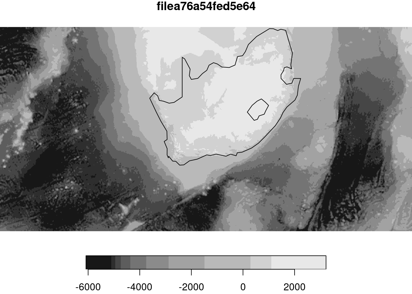
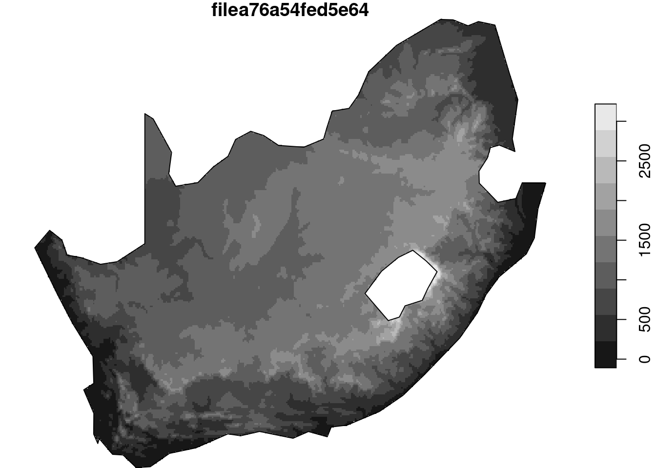
stars object with 2 dimensions and 1 attribute
attribute(s):
                    Min. 1st Qu. Median      Mean 3rd Qu. Max.
filea76a54fed5e64  -6084   -4853  -3745 -2750.098    -155 3218
dimension(s):
  from   to  offset      delta refsys point x/y
x    1 1054       0  0.0426784 WGS 84  TRUE [x]
y    1  446 -21.943 -0.0426784 WGS 84  TRUE [y]
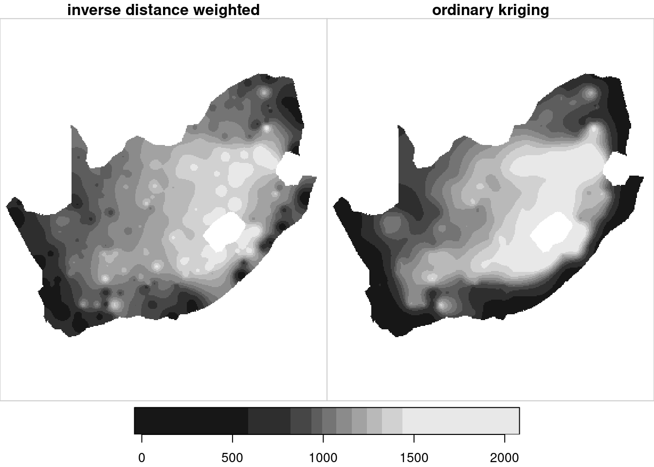
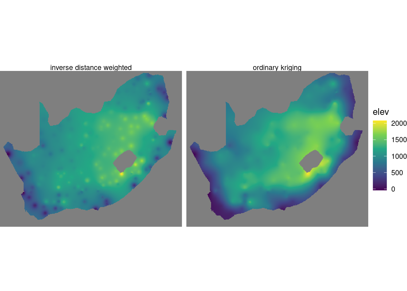
Geostatistical data

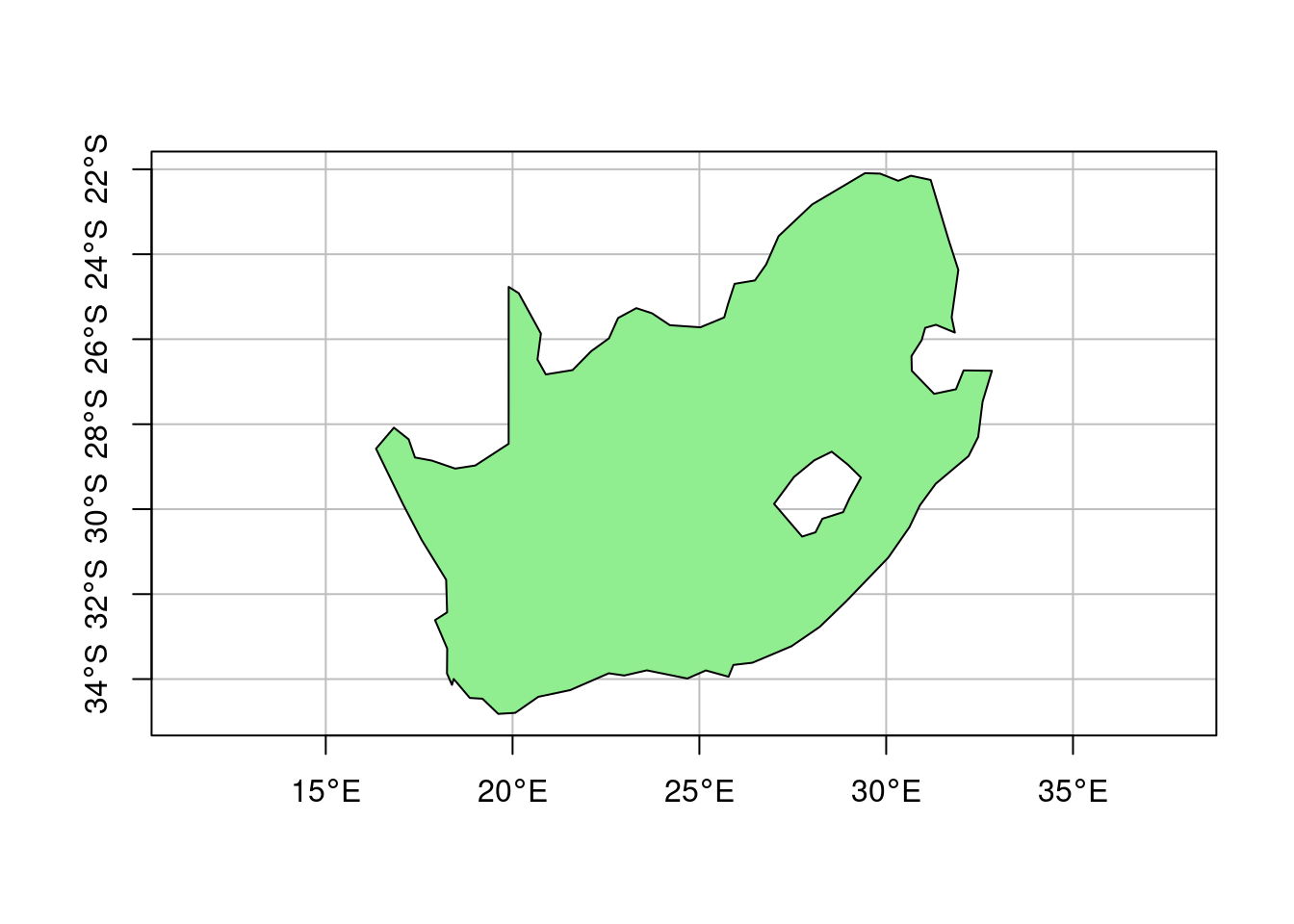
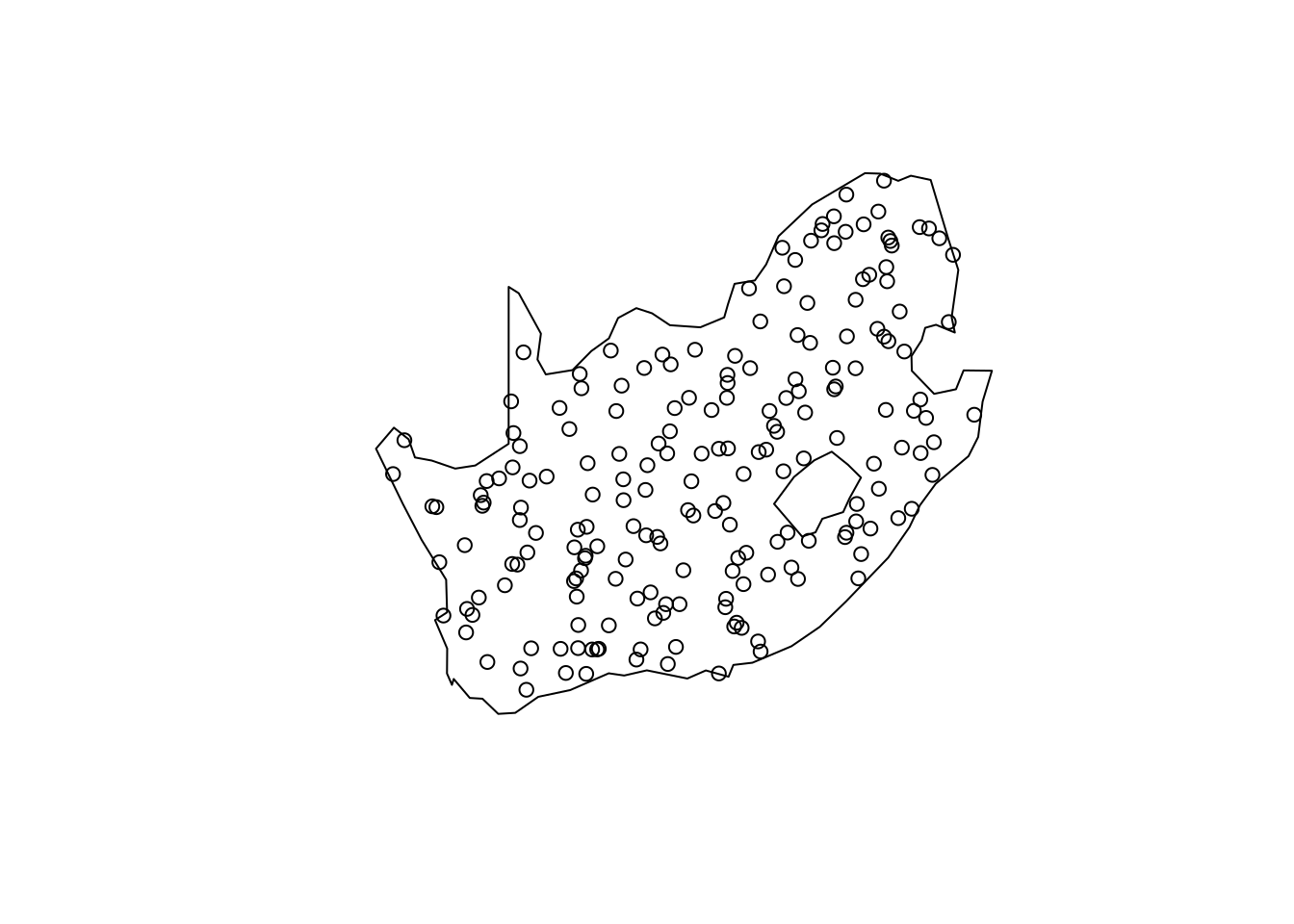
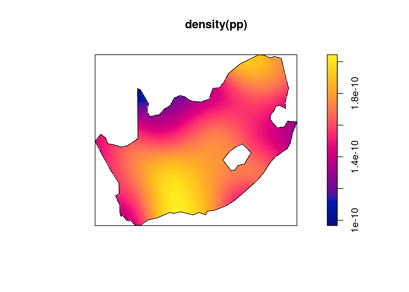
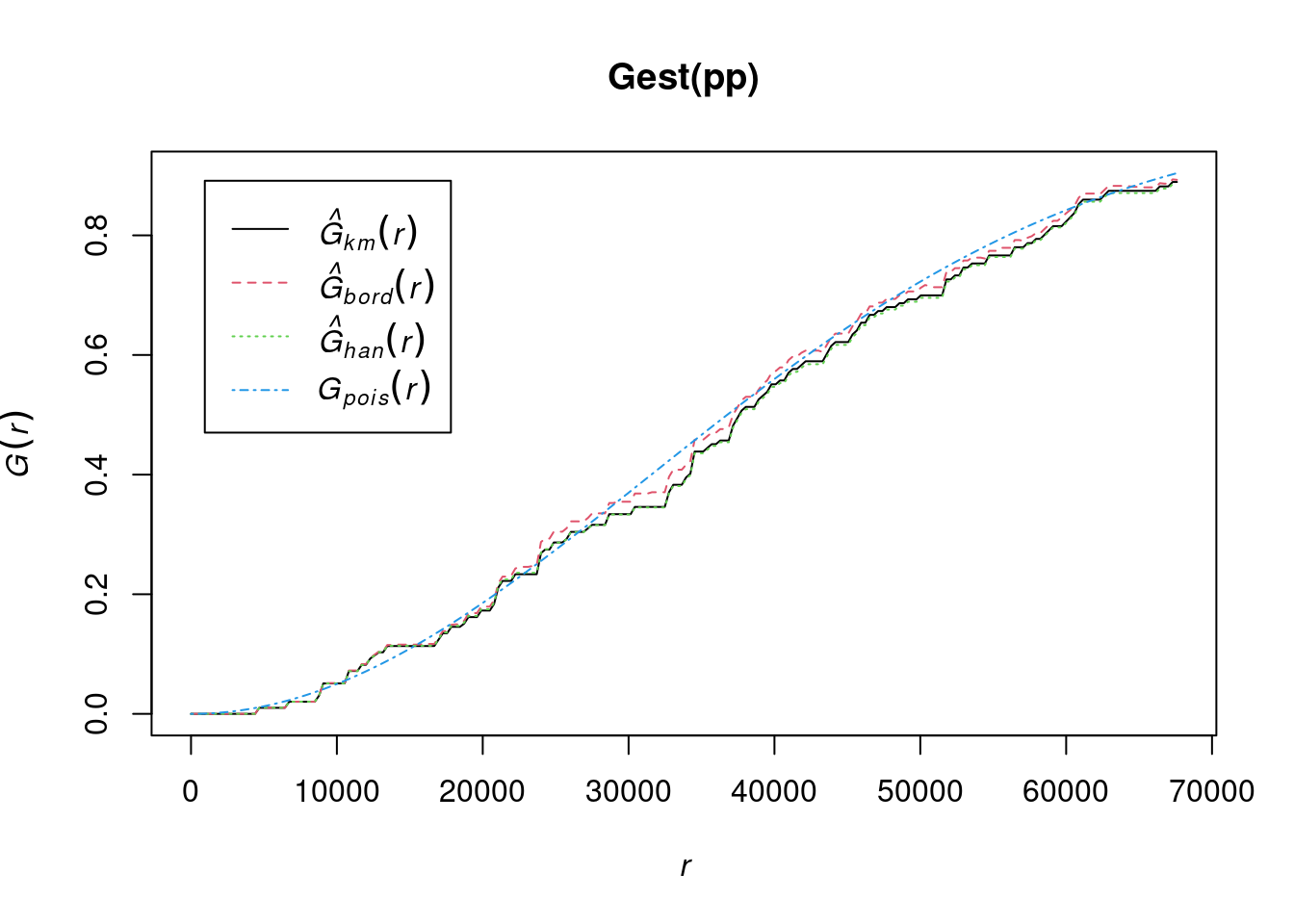
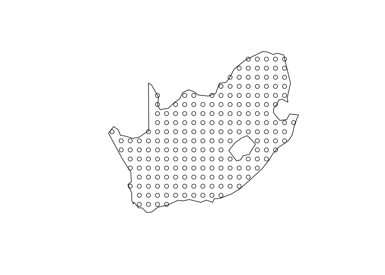
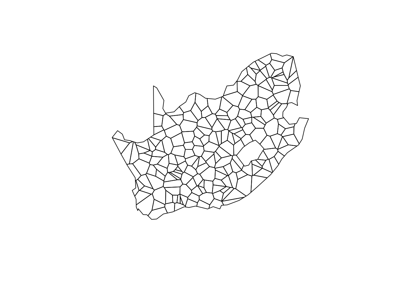
Suppose we have 200 elevation observations, randomly sampled over the area of SA:

set.seed(1331) # remove this if you want different random points
pts = st_sample(sa, 200)
st_geometry(sa) |> plot()
plot(pts, add = TRUE)

elev.200 = st_extract(elev, pts) |> setNames(c("elev", "geometry")) |> 
  st_transform(utm34s)

Inverse distance interpolation:

elev[sa] |> st_warp(crs = utm34s) -> elev.utm
library(gstat)
k = idw(elev ~ 1, elev.200, elev.utm)
[inverse distance weighted interpolation]
plot(k, reset = FALSE)
plot(elev.200, add = TRUE, pch = 3, col = 'green')

Ordinary kriging

v = variogram(elev~1, elev.200)
v.fit = fit.variogram(v, vgm(1e5, "Exp", 1e5))
plot(v, v.fit)

kr = krige(elev ~ 1, elev.200, elev.utm, v.fit)
[using ordinary kriging]
plot(kr, reset = FALSE)
plot(elev.200, add = TRUE, pch = 3, col = 'green')

Side-by-side comparison idw - OK:

kr$idw = k$var1.pred # copy over raster layer
kr$ok = kr$var1.pred # copy over raster layer
kr[c("idw", "ok")] |> 
  setNames(c("inverse distance weighted", "ordinary kriging")) |> 
  merge() |> 
  plot()

Doing the same with ggplot2:

kr[c("idw", "ok")] |> 
  setNames(c("inverse distance weighted", "ordinary kriging")) |> 
  merge() |> setNames("elev") -> d
library(ggplot2)
ggplot() + geom_stars(data = d) +
        facet_wrap(~attributes) +
        coord_equal() +
        theme_void() +
        scale_x_discrete(expand = c(0,0)) +
        scale_y_discrete(expand = c(0,0)) +
        scale_fill_viridis_c()

Or mapview:

mapview(d[,,,1]) + mapview(d[,,,2])

Point patterns

Although we know that elev.200 is a random sample, we can do some point pattern analysis on it:

library(spatstat)
Loading required package: spatstat.data
Loading required package: spatstat.geom
spatstat.geom 3.0-3
Loading required package: spatstat.random
spatstat.random 3.0-0
Loading required package: spatstat.explore
Loading required package: nlme

Attaching package: 'nlme'
The following object is masked from 'package:dplyr':

    collapse
spatstat.explore 3.0-0

Attaching package: 'spatstat.explore'
The following object is masked from 'package:gstat':

    idw
Loading required package: spatstat.model
Loading required package: rpart
spatstat.model 3.0-0
Loading required package: spatstat.linnet
spatstat.linnet 2.999-999.021

spatstat 2.999-999.010       (nickname: 'Watch this space') 
For an introduction to spatstat, type 'beginner' 
pts = st_geometry(elev.200)
st_geometry(sa) |> st_transform(utm34s) -> sa.utm
c(sa.utm, pts)
Geometry set for 201 features 
Geometry type: GEOMETRY
Dimension:     XY
Bounding box:  xmin: 44478.86 ymin: 6146428 xmax: 1681464 ymax: 7533016
Projected CRS: Cape / UTM zone 34S
First 5 geometries:
MULTIPOLYGON (((1525272 6717455, 1504676 670302...
POINT (335632.9 6753557)
POINT (1601722 7302046)
POINT (814353.7 6316993)
POINT (746946.7 6610462)
c(sa.utm, pts) |> as.ppp() -> pp
plot(density(pp))
plot(sa.utm, add = TRUE)

We can explore the density of point by comparing to completely spatially random (CSR):

Gest(pp) |> plot() # nearest neighbour distance

Kest(pp) |> plot() # lamba * K(r) = # of points expected in a radius r

st_sample(sa.utm, 200, type = "regular") |> st_geometry() -> r
c(sa.utm, r) |> as.ppp() -> pp.r
Gest(pp.r) |> plot() # nearest neighbour distance

Kest(pp.r) |> plot() # lamba * K(r) = # of points expected in a radius r

plot(st_geometry(sa.utm))
plot(pp.r, add = TRUE)

Area/lattice data

We will create some artificial lattice data by first creating a voronoi tesselation using the 200 random points:

st_geometry(elev.200) |> 
  st_combine() |> 
  st_voronoi() |> 
  st_collection_extract("POLYGON") -> v
plot(v)

We will constrain this to the area of SA:

v2 = st_intersection(sa.utm, v)
plot(v2)

and compute mean elevation for each of the polygons:

aggregate(elev.utm, v2, mean, na.rm = TRUE) |> st_as_sf() -> v2.elev
names(v2.elev)[1] = "elev"
plot(v2.elev)

Next, we can compute spatial neigbours for each polygon, using spdep::poly2nb():

library(spdep)
Loading required package: sp
Loading required package: spData
v2.elev |> poly2nb() -> nb
nb
Neighbour list object:
Number of regions: 200 
Number of nonzero links: 1074 
Percentage nonzero weights: 2.685 
Average number of links: 5.37 
plot(st_geometry(v2.elev))
v2.elev |> st_geometry() |> st_centroid() |> st_coordinates() -> cc
plot(nb, coords = cc, add = TRUE, col = 'orange')

and, using row-standardised weights list

lw = nb2listw(nb)

we can compute Moran’s I, first for random data:

set.seed(1)
v2.elev$random = rnorm(nrow(v2.elev))
moran.test(v2.elev$random, lw)

    Moran I test under randomisation

data:  v2.elev$random  
weights: lw    

Moran I statistic standard deviate = -1.0595, p-value = 0.8553
alternative hypothesis: greater
sample estimates:
Moran I statistic       Expectation          Variance 
     -0.051330515      -0.005025126       0.001910166 

then for actual (elevation) data:

moran.test(v2.elev$elev, lw)

    Moran I test under randomisation

data:  v2.elev$elev  
weights: lw    

Moran I statistic standard deviate = 16.618, p-value < 2.2e-16
alternative hypothesis: greater
sample estimates:
Moran I statistic       Expectation          Variance 
      0.721435742      -0.005025126       0.001911137 
v2.elev$x = cc[,1]
v2.elev$y = cc[,2]
lm(elev~1, v2.elev) |> lm.morantest(lw)

    Global Moran I for regression residuals

data:  
model: lm(formula = elev ~ 1, data = v2.elev)
weights: lw

Moran I statistic standard deviate = 16.63, p-value < 2.2e-16
alternative hypothesis: greater
sample estimates:
Observed Moran I      Expectation         Variance 
     0.721435742     -0.005025126      0.001908353 
lm(elev~x+y, v2.elev) |> lm.morantest(lw)

    Global Moran I for regression residuals

data:  
model: lm(formula = elev ~ x + y, data = v2.elev)
weights: lw

Moran I statistic standard deviate = 16.404, p-value < 2.2e-16
alternative hypothesis: greater
sample estimates:
Observed Moran I      Expectation         Variance 
     0.689267331     -0.014895347      0.001842773 

Non-spatial and spatial regression model, using x and y as regressors, can be computed; non-spatial uses lm():

lm(elev~x+y, v2.elev) |> summary()

Call:
lm(formula = elev ~ x + y, data = v2.elev)

Residuals:
     Min       1Q   Median       3Q      Max 
-1095.16  -215.09    48.33   288.65   782.61 

Coefficients:
             Estimate Std. Error t value Pr(>|t|)   
(Intercept) 5.157e+02  6.178e+02   0.835  0.40484   
x           2.591e-04  8.248e-05   3.141  0.00194 **
y           4.611e-05  9.655e-05   0.478  0.63346   
---
Signif. codes:  0 '***' 0.001 '**' 0.01 '*' 0.05 '.' 0.1 ' ' 1

Residual standard error: 370.1 on 197 degrees of freedom
Multiple R-squared:  0.07773,   Adjusted R-squared:  0.06837 
F-statistic: 8.302 on 2 and 197 DF,  p-value: 0.0003454

Spatial error model can use one of many (see Ch 17), here errorsarlm():

library(spatialreg)
Loading required package: Matrix

Attaching package: 'spatialreg'
The following objects are masked from 'package:spdep':

    get.ClusterOption, get.coresOption, get.mcOption,
    get.VerboseOption, get.ZeroPolicyOption, set.ClusterOption,
    set.coresOption, set.mcOption, set.VerboseOption,
    set.ZeroPolicyOption
errorsarlm(elev~x+y, v2.elev, listw = lw, Durbin=FALSE) |> summary()

Call:errorsarlm(formula = elev ~ x + y, data = v2.elev, listw = lw, 
    Durbin = FALSE)

Residuals:
     Min       1Q   Median       3Q      Max 
-514.031  -88.375  -10.678  103.665  578.148 

Type: error 
Coefficients: (asymptotic standard errors) 
               Estimate  Std. Error z value  Pr(>|z|)
(Intercept) -5.8857e+03  2.9743e+03 -1.9788 0.0478334
x           -1.5065e-03  4.4506e-04 -3.3849 0.0007119
y            1.1575e-03  4.2643e-04  2.7144 0.0066387

Lambda: 0.9742, LR test value: 255.62, p-value: < 2.22e-16
Asymptotic standard error: 0.011728
    z-value: 83.068, p-value: < 2.22e-16
Wald statistic: 6900.3, p-value: < 2.22e-16

Log likelihood: -1337.232 for error model
ML residual variance (sigma squared): 26159, (sigma: 161.74)
Number of observations: 200 
Number of parameters estimated: 5 
AIC: 2684.5, (AIC for lm: 2938.1)