Code
library(rnaturalearth)
library(sf)
# Linking to GEOS 3.12.1, GDAL 3.8.4, PROJ 9.4.0; sf_use_s2() is TRUE
par(mar = c(2,2,0,0) + .1)
ne_countries() |> st_geometry() |> plot(axes=TRUE)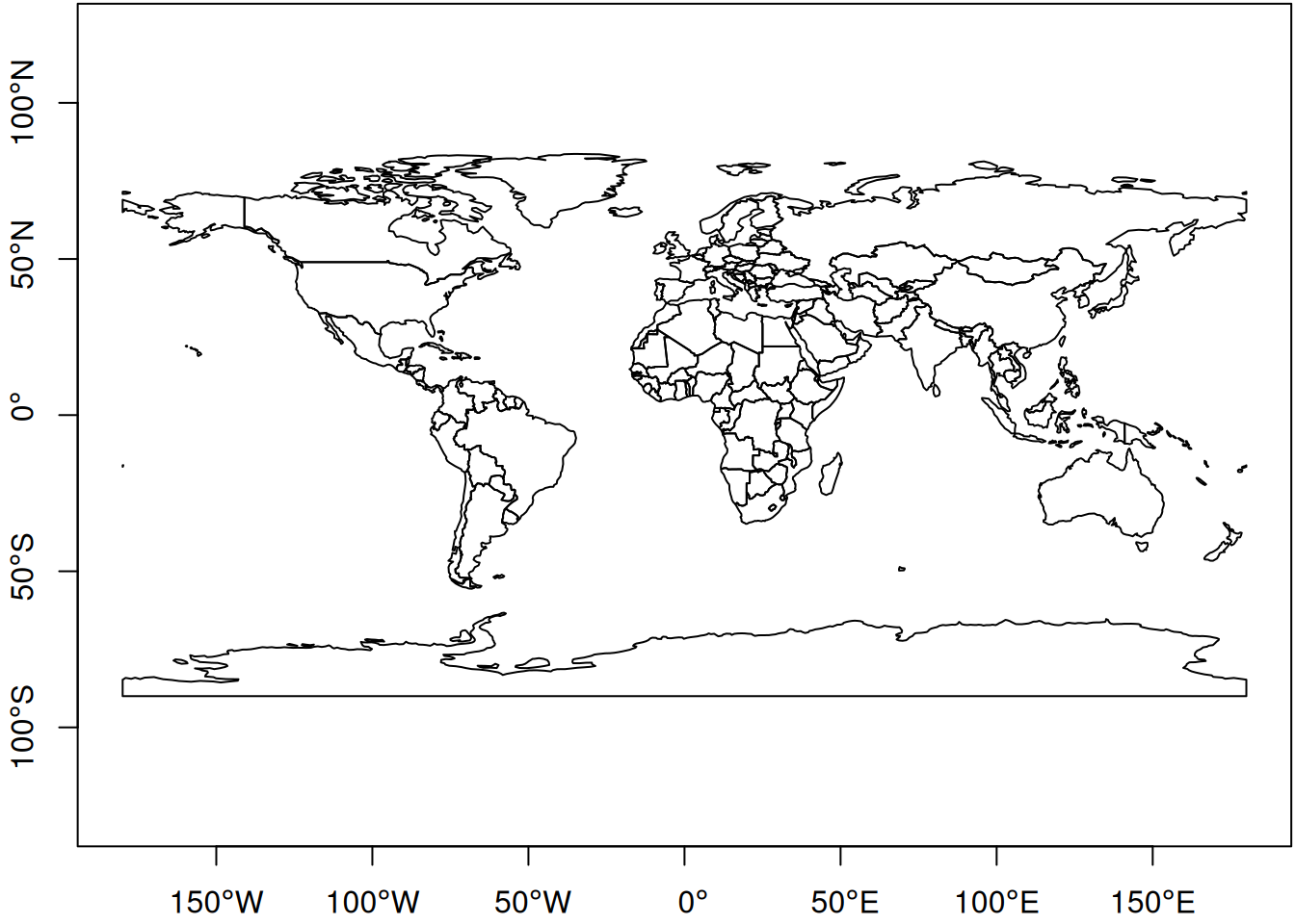
library(rnaturalearth)
library(sf)
# Linking to GEOS 3.12.1, GDAL 3.8.4, PROJ 9.4.0; sf_use_s2() is TRUE
par(mar = c(2,2,0,0) + .1)
ne_countries() |> st_geometry() |> plot(axes=TRUE)
“Simple features” comes from simple feature access, an OGC standard. OGC stands for “Open Geospatial Consortium” and is a standardisation body; many OGC standards become ISO standards (for whatever it is worth!).
A feature is a “thing” that has
“Simple” in “simple feature” refers to the property that geometries are points, lines or polygons, and that lines and polygon boundaries consists of sequences of points connected with straight lines (edges), and that edges do not cross other edges (do not self-intersect). Polygons consist of an outer (closed) ring with zero or more inner (closed) rings denoting holes.
Simple feature geometries are zero-dimensional (points), one-dimensional (linestrings), or two-dimensional (polygons). Each geometry has an interior (I), a boundary (B) and an exterior (E). For polygons this is trivial, but
sf and stars
sf provides classes and methods for simple features
sf stores data in data.frames with a list-column (of class sfc) that holds the geometries“Simple Feature Access” is an open standard for data with vector geometries. It defines a set of classes for geometries and operations on them.
sf start with st_?sf operators, how to understand?Package sf has objects at three nested “levels”:
sfg: a single geometry (without coordinate reference system); contained in:
sfc: a set of sfg geometries (list), with a coordinate reference system and bounding box; contained in:
sf: a data.frame or tibble with at least one geometry (sfc) column
Operations not involving geometry (data.frame; base R; tidyverse)
sf class is sticky!as.data.frame or as_tibble to strip the sf class labelOperations involving only geometry
TRUE/FALSE)
sgbp, which is a sparse logical matrix representation
by_element = FALSE
Operations involving geometry and attributes
st_joinaggregatest_interpolate_aw: requires expression whether variable is spatially extensive or intensive
sf and spatstat
We can try to convert an sf object to a ppp (point pattern object in spatstat):
library(sf)
library(spatstat)
# Loading required package: spatstat.data
# Loading required package: spatstat.univar
# spatstat.univar 3.1-1
# Loading required package: spatstat.geom
# spatstat.geom 3.3-4
# Loading required package: spatstat.random
# spatstat.random 3.3-2
# Loading required package: spatstat.explore
# Loading required package: nlme
# spatstat.explore 3.3-4
# Loading required package: spatstat.model
# Loading required package: rpart
# spatstat.model 3.3-3
# Loading required package: spatstat.linnet
# spatstat.linnet 3.2-3
#
# spatstat 3.3-0
# For an introduction to spatstat, type 'beginner'
demo(nc, echo = FALSE, ask = FALSE)
pts = st_centroid(st_geometry(nc))
as.ppp(pts) # ???
# Error: Only projected coordinates may be converted to spatstat
# class objects
Note that sf interprets a NA CRS as: flat, projected (Cartesian) space.
starsPackages stars is a package for (dense) array data, where array dimensions are associated with space and/or time (spatial time series, data cubes). It is built for simplicity (pure R), and for maximum integration with sf.
R’s array is very powerful, but its metadata (dimnames) is restricted to character vectors.
A stars object
dimensions attribute with all the metadata of the dimensions (offset, cellsize, units, reference system, point/block support)library(stars)
# Loading required package: abind
st_as_stars() # default: 1 degree global Cartesian grid
# stars object with 2 dimensions and 1 attribute
# attribute(s):
# Min. 1st Qu. Median Mean 3rd Qu. Max.
# values 0 0 0 0 0 0
# dimension(s):
# from to offset delta refsys x/y
# x 1 360 -180 1 WGS 84 (CRS84) [x]
# y 1 180 90 -1 WGS 84 (CRS84) [y]Valid polygons are polygons with several geometrical constraints, such as
In particular the last condition is often dropped, as the order of the rings already denotes their role, and winding can easily reversed. An exception of this is polygons on the sphere, where both inside and outside have a limited area.
The intersection of two geometries is the set of points they have in common. This set can be empty (no points), 0-, 1-, or 2-dimensional. The DE-9IM defines the relation between two geometries as the intersection of I, B and E of the first and the second geometry (hence: 9, see https://r-spatial.org/book/03-Geometries.html#fig-de9im). The values can be F (empty), 0, 1 or 2 (dimension if not empty), or T (not empty: any of 0, 1 or 2). Using the resulting encoding (the relation), one can define special predicates, such as
and many more on; one can also define custom queries with a specific pattern, e.g.:
0FFFFFFF2.We often work with polygon data that form a polygon coverage, which is a tesselation of an area of interest, e.g.
When representing the polygons as a set of outer rings, it is hard to see whether there are no overlaps, and no gaps between polygons. Such overlaps or gaps could result from generalisation of polygon boundaries, one-by-one, and not by first identifying a common boundary and then generalizing that.
“True” geographic information systems (e.g. ArcGIS or GRASS GIS) use a topological representation of geometries that consists of edge nodes and (outer and inner) boundaries, and can do such simplifications without creating overlaps or gaps.
Another challenge is that polygon coverages represented as a set of simple feature polygons do not uniquely assign all points to a single unit. Points on a boundary common to two geometries intersect with both, there is no geometric argument to assign them unambiguously to only one of them.
Finally, as the Earth is round, the use of straight lines is problematic:
In addition to vector (point/line/polygon) data, we also have raster data. For regular rasters, space is cut into square cells, aligned with \(x\) and \(y\). Raster spaces can tesselate, see here.
In addition to regular rasters, we have rotated, sheared, rectilinear and curvilinear rasters. The raster space is primarily flat, so any time we use it model data of the Earth surface, we violate the constant raster cell size concept. Many data are distributed as regular rasters in geodetic coordinates (long/lat space, e.g., 0.25 degree raster cells), mostly for convienience (of who?)
Discrete global grids are (semi-)regular tesselations of the Earth surface, using squares, triangles, or hexagons. Examples are:
Interestingly, computer screens are raster devices, so any time we do view vector data on a computer screen, a rasterization has taken place.
Data cubes are array data with one or more dimensions associated with space or geometry. The degenerate example is a one-dimensional array (or collection thereof), which we have in a table or data.frame. The canonical example of array data is raster data, or a time series thereof.
Further examples include:
library(sf)
no2 <- read.csv(system.file("external/no2.csv",
    package = "gstat"))
crs <- st_crs("EPSG:32632")
st_as_sf(no2, crs = "OGC:CRS84", coords =
    c("station_longitude_deg", "station_latitude_deg")) |>
    st_transform(crs) -> no2.sf
library(ggplot2)
# plot(st_geometry(no2.sf))
read_sf("de_nuts1.gpkg") |>
  st_transform(crs) -> de
ggplot() + geom_sf(data = de) +
    geom_sf(data = no2.sf, mapping = aes(col = NO2))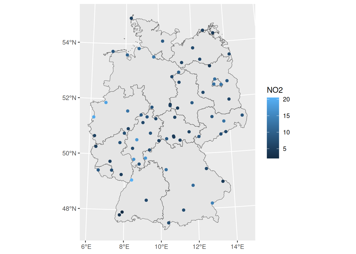
# https://en.wikipedia.org/wiki/List_of_NUTS_regions_in_the_European_Union_by_GDP
de$GDP_percap = c(45200, 46100, 37900, 27800, 49700, 64700, 45000, 26700, 36500, 38700, 35700, 35300, 29900, 27400, 32400, 28900)
ggplot() + geom_sf(data = de) +
    geom_sf(data = de, mapping = aes(fill = GDP_percap)) +
    geom_sf(data = st_cast(de, "MULTILINESTRING"), col = 'white')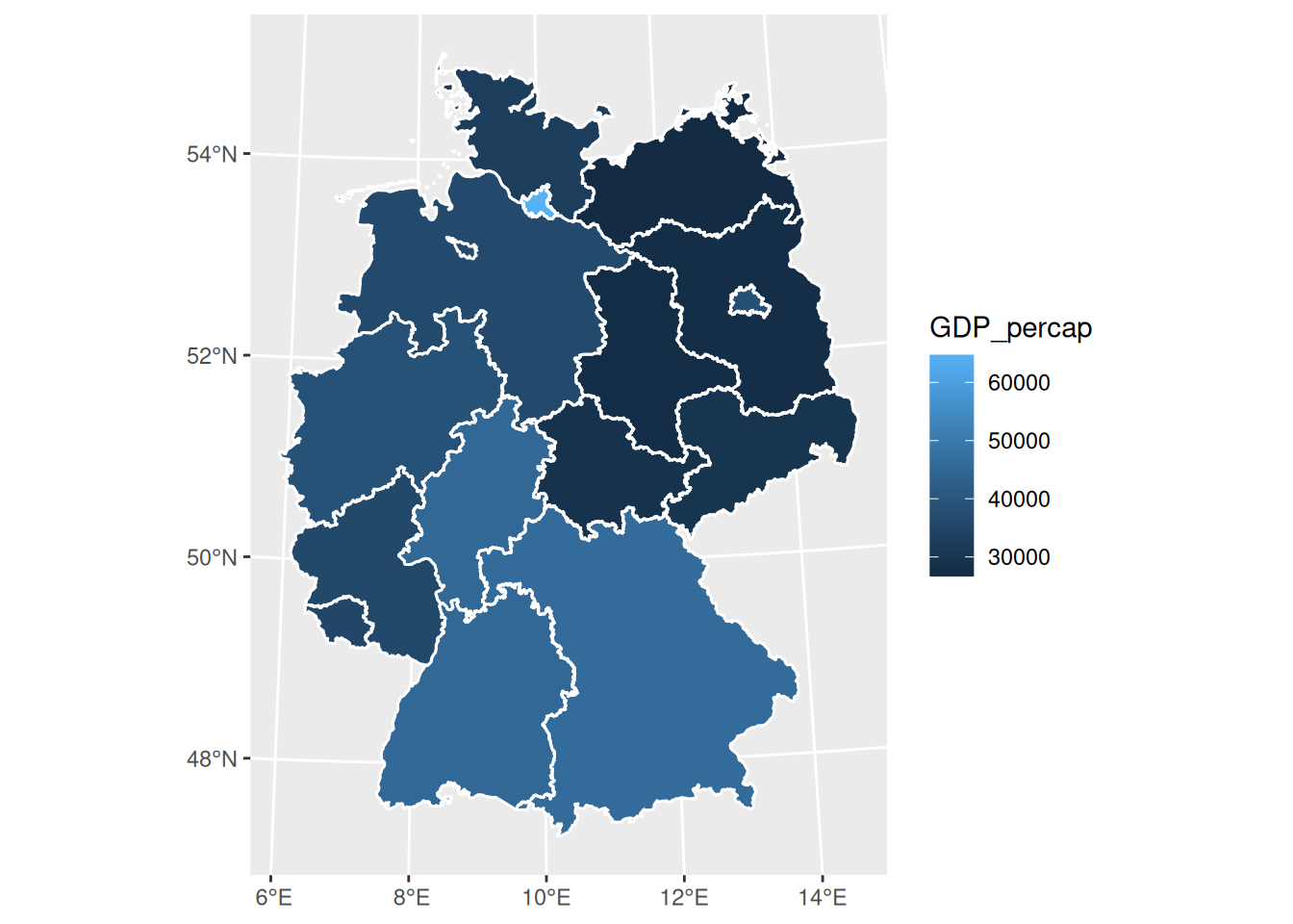
# from: https://r-spatial.org/r/2017/08/28/nest.html
library(tidyverse)
# ── Attaching core tidyverse packages ──────────── tidyverse 2.0.0 ──
# ✔ dplyr     1.1.4     ✔ readr     2.1.5
# ✔ forcats   1.0.0     ✔ stringr   1.5.1
# ✔ lubridate 1.9.4     ✔ tibble    3.2.1
# ✔ purrr     1.0.2     ✔ tidyr     1.3.1
# ── Conflicts ────────────────────────────── tidyverse_conflicts() ──
# ✖ dplyr::collapse() masks nlme::collapse()
# ✖ dplyr::filter()   masks stats::filter()
# ✖ dplyr::lag()      masks stats::lag()
# ℹ Use the conflicted package (<http://conflicted.r-lib.org/>) to force all conflicts to become errors
storms.sf <- storms %>%
    st_as_sf(coords = c("long", "lat"), crs = 4326)
storms.sf <- storms.sf %>%
    mutate(time = as.POSIXct(paste(paste(year,month,day, sep = "-"),
                                   paste(hour, ":00", sep = "")))) %>%
    select(-month, -day, -hour)
storms.nest <- storms.sf %>% group_by(name, year) %>% nest
to_line <- function(tr) st_cast(st_combine(tr), "LINESTRING") %>% .[[1]]
tracks <- storms.nest %>% pull(data) %>% map(to_line) %>% st_sfc(crs = 4326)
storms.tr <- storms.nest %>% select(-data) %>% st_sf(geometry = tracks)
storms.tr %>% ggplot(aes(color = year)) + geom_sf()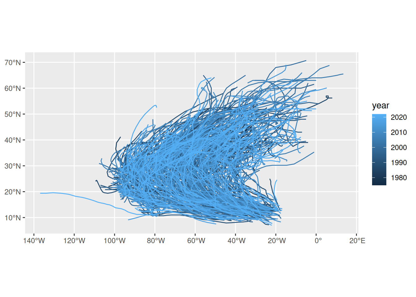
In design-based statistics, randomness comes from random sampling. Consider an area \(B\), from which we take samples \[z(s), s \in B,\] with \(s\) a location for instance two-dimensional: \(s_i = \{x_i,y_i\}\). If we select the samples randomly, we can consider \(S \in B\) a random variable, and \(z(S)\) a random sample. Note the randomness in \(S\), not in \(z\).
Two variables \(z(S_1)\) and \(z(S_2)\) are independent if \(S_1\) and \(S_2\) are sampled independently. For estimation we need to know the inclusion probabilities, which need to be non-negative for every location.
If inclusion probabilities are constant (simple random sampling; or complete spatial randomness: day 2, point patterns) then we can estimate the mean of \(Z(B)\) by the sample mean \[\frac{1}{n}\sum_{j=1}^n z(s_j).\] This also predicts the value of a randomly chosen observation \(z(S)\). It cannot be used to predict the value \(z(s_0)\) for a non-randomly chosen location \(s_0\); for this we need a model.
Model-based statistics assumes randomness in the measured responses; consider a regression model \(y = X\beta + e\), where \(e\) is a random variable and as a consequence \(y\), the response variable is a random variable. In the spatial context we replace \(y\) with \(z\), and capitalize it to indicate it is a random variable, and write \[Z(s) = X(s)\beta + e(s)\] to stress that
In the regression literature this is called a (linear) mixed model, because \(e\) is not i.i.d. If \(e(s)\) contains an iid component \(\epsilon\) we can write this as
\[Z(s) = X(s)\beta + w(s) + \epsilon\]
with \(w(s)\) the spatial signal, and \(\epsilon\) a noise compenent e.g. due to measurement error.
Predicting \(Z(s_0)\) will involve (GLS) estimation of \(\beta\), but also prediction of \(e(s_0)\) using correlated, nearby observations (day 3: geostatistics).
ne_countries() dataset, imported above?ne_countries to Plate Carrée, and plot it with axes=TRUE. What has changed? (Hint: st_crs() accepts a proj string to define a coordinate reference system (CRS); st_transform() transforms a dataset to a new CRS.)+proj=ortho; what went wrong?Next: continue with the exercises of Chapter 3 of “Spatial Data Science: with applications in R”, then those of Chapter 6.