library(spatstat)
# Loading required package: spatstat.data
# Loading required package: spatstat.univar
# spatstat.univar 3.1-1
# Loading required package: spatstat.geom
# spatstat.geom 3.3-4
# Loading required package: spatstat.random
# spatstat.random 3.3-2
# Loading required package: spatstat.explore
# Loading required package: nlme
# spatstat.explore 3.3-4
# Loading required package: spatstat.model
# Loading required package: rpart
# spatstat.model 3.3-3
# Loading required package: spatstat.linnet
# spatstat.linnet 3.2-3
#
# spatstat 3.3-0
# For an introduction to spatstat, type 'beginner'
set.seed(1357)
CRS = rpoispp(100)
ppi = rpoispp(function(x,y,...) 500 * x)4 prediction and simulation
4.1 point patterns:
Fitting models
After generating the CRS and inhom. Poisson patterns:
we can fit an inhomogeneous Poisson point process to these patterns: # assuming Inhomogeneous Poisson:
ppm(CRS, ~x)
# Nonstationary Poisson process
# Fitted to point pattern dataset 'CRS'
#
# Log intensity:  ~x
#
# Fitted trend coefficients:
# (Intercept)           x
#       4.705      -0.143
#
#             Estimate  S.E. CI95.lo CI95.hi Ztest   Zval
# (Intercept)    4.705 0.194   4.326   5.085   *** 24.291
# x             -0.143 0.342  -0.812   0.527       -0.418
ppm(ppi, ~x)
# Nonstationary Poisson process
# Fitted to point pattern dataset 'ppi'
#
# Log intensity:  ~x
#
# Fitted trend coefficients:
# (Intercept)           x
#        4.23        2.14
#
#             Estimate  S.E. CI95.lo CI95.hi Ztest  Zval
# (Intercept)     4.23 0.177    3.89    4.58   *** 23.87
# x               2.14 0.248    1.66    2.63   ***  8.64
or fit an Inhomogeneous clustered point process to data:
# assuming Inhomogeneous clustered, Thomas process:
kppm(CRS, ~x) |> summary()
# Inhomogeneous cluster point process model
# Fitted to point pattern dataset 'CRS'
# Fitted by minimum contrast
#   Summary statistic: inhomogeneous K-function
# Minimum contrast fit (object of class "minconfit")
# Model: Thomas process
# Fitted by matching theoretical K function to CRS
#
# Internal parameters fitted by minimum contrast ($par):
#    kappa   sigma2
# 1.46e+06 2.36e+01
#
# Fitted cluster parameters:
#    kappa    scale
# 1.46e+06 4.86e+00
# Mean cluster size:  [pixel image]
#
# Converged successfully after 47 function evaluations
#
# Starting values of parameters:
#    kappa   sigma2
# 1.03e+02 8.98e-03
# Domain of integration: [ 0 , 0.25 ]
# Exponents: p= 2, q= 0.25
#
# ----------- TREND  -----
# Point process model
# Fitted to data: X
# Fitting method: maximum likelihood (Berman-Turner approximation)
# Model was fitted using glm()
# Algorithm converged
# Call:
# ppm.ppp(Q = X, trend = trend, rename.intercept = FALSE, covariates = covariates,
#     covfunargs = covfunargs, use.gam = use.gam, forcefit = TRUE,
#     improve.type = ppm.improve.type, improve.args = ppm.improve.args,
#     nd = nd, eps = eps)
# Edge correction: "border"
#   [border correction distance r = 0 ]
# --------------------------------------------------------------------
# Quadrature scheme (Berman-Turner) = data + dummy + weights
#
# Data pattern:
# Planar point pattern:  103 points
# Average intensity 103 points per square unit
# Window: rectangle = [0, 1] x [0, 1] units
# Window area = 1 square unit
#
# Dummy quadrature points:
#      32 x 32 grid of dummy points, plus 4 corner points
#      dummy spacing: 0.0312 units
#
# Original dummy parameters: =
# Planar point pattern:  1028 points
# Average intensity 1030 points per square unit
# Window: rectangle = [0, 1] x [0, 1] units
# Window area = 1 square unit
# Quadrature weights:
#      (counting weights based on 32 x 32 array of rectangular tiles)
# All weights:
#   range: [0.000244, 0.000977] total: 1
# Weights on data points:
#   range: [0.000244, 0.000488] total: 0.0483
# Weights on dummy points:
#   range: [0.000244, 0.000977] total: 0.952
# --------------------------------------------------------------------
# FITTED :
#
# Nonstationary Poisson process
#
# ---- Intensity: ----
#
# Log intensity: ~x
#
# Fitted trend coefficients:
# (Intercept)           x
#       4.705      -0.143
#
#             Estimate  S.E. CI95.lo CI95.hi Ztest   Zval
# (Intercept)    4.705 0.194   4.326   5.085   *** 24.291
# x             -0.143 0.342  -0.812   0.527       -0.418
#
# ----------- gory details -----
#
# Fitted regular parameters (theta):
# (Intercept)           x
#       4.705      -0.143
#
# Fitted exp(theta):
# (Intercept)           x
#     110.521       0.867
#
# ----------- CLUSTER  -----------
# Model: Thomas process
#
# Fitted cluster parameters:
#    kappa    scale
# 1.46e+06 4.86e+00
# Mean cluster size:  [pixel image]
#
# Final standard error and CI
# (allowing for correlation of cluster process):
#             Estimate  S.E. CI95.lo CI95.hi Ztest   Zval
# (Intercept)    4.705 0.194   4.326   5.085   *** 24.291
# x             -0.143 0.342  -0.812   0.527       -0.418
#
# ----------- cluster strength indices ----------
# Mean sibling probability 2.31e-09
# Count overdispersion index (on original window): 1
# Cluster strength: 2.31e-09
#
# Spatial persistence index (over window): 0.979
#
# Bound on distance from Poisson process (over window): 2.66e-05
#    = min (1, 0.0156, 0.0073, 2.66e-05, 0.00495)
#
# >>> The Poisson process is a better fit <<<kppm(ppi, ~x) |> summary()
# Inhomogeneous cluster point process model
# Fitted to point pattern dataset 'ppi'
# Fitted by minimum contrast
# Summary statistic: inhomogeneous K-function
# Minimum contrast fit (object of class "minconfit")
# Model: Thomas process
# Fitted by matching theoretical K function to ppi
#
# Internal parameters fitted by minimum contrast ($par):
# kappa sigma2
# 1.76e+03 5.85e-03
#
# Fitted cluster parameters:
# kappa scale
# 1.76e+03 7.65e-02
# Mean cluster size: [pixel image]
#
# Converged successfully after 47 function evaluations
#
# Starting values of parameters:
# kappa sigma2
# 2.42e+02 4.14e-03
# Domain of integration: [ 0 , 0.25 ]
# Exponents: p= 2, q= 0.25
#
# ----------- TREND -----
# Point process model
# Fitted to data: X
# Fitting method: maximum likelihood (Berman-Turner approximation)
# Model was fitted using glm()
# Algorithm converged
# Call:
# ppm.ppp(Q = X, trend = trend, rename.intercept = FALSE, covariates = covariates,
# covfunargs = covfunargs, use.gam = use.gam, forcefit = TRUE,
# improve.type = ppm.improve.type, improve.args = ppm.improve.args,
# nd = nd, eps = eps)
# Edge correction: "border"
# [border correction distance r = 0 ]
# --------------------------------------------------------------------
# Quadrature scheme (Berman-Turner) = data + dummy + weights
#
# Data pattern:
# Planar point pattern: 242 points
# Average intensity 242 points per square unit
# Window: rectangle = [0, 1] x [0, 1] units
# Window area = 1 square unit
#
# Dummy quadrature points:
# 40 x 40 grid of dummy points, plus 4 corner points
# dummy spacing: 0.025 units
#
# Original dummy parameters: =
# Planar point pattern: 1604 points
# Average intensity 1600 points per square unit
# Window: rectangle = [0, 1] x [0, 1] units
# Window area = 1 square unit
# Quadrature weights:
# (counting weights based on 40 x 40 array of rectangular tiles)
# All weights:
# range: [0.000156, 0.000625] total: 1
# Weights on data points:
# range: [0.000156, 0.000312] total: 0.072
# Weights on dummy points:
# range: [0.000156, 0.000625] total: 0.928
# --------------------------------------------------------------------
# FITTED :
#
# Nonstationary Poisson process
#
# ---- Intensity: ----
#
# Log intensity: ~x
#
# Fitted trend coefficients:
# (Intercept) x
# 4.23 2.14
#
# Estimate S.E. CI95.lo CI95.hi Ztest Zval
# (Intercept) 4.23 0.177 3.89 4.58 *** 23.87
# x 2.14 0.248 1.66 2.63 *** 8.64
#
# ----------- gory details -----
#
# Fitted regular parameters (theta):
# (Intercept) x
# 4.23 2.14
#
# Fitted exp(theta):
# (Intercept) x
# 68.91 8.53
#
# ----------- CLUSTER -----------
# Model: Thomas process
#
# Fitted cluster parameters:
# kappa scale
# 1.76e+03 7.65e-02
# Mean cluster size: [pixel image]
#
# Final standard error and CI
# (allowing for correlation of cluster process):
# Estimate S.E. CI95.lo CI95.hi Ztest Zval
# (Intercept) 4.23 0.183 3.87 4.59 *** 23.12
# x 2.14 0.259 1.64 2.65 *** 8.28
#
# ----------- cluster strength indices ----------
# Mean sibling probability 0.00766
# Count overdispersion index (on original window): 1.14
# Cluster strength: 0.00772
#
# Spatial persistence index (over window): 0
#
# Bound on distance from Poisson process (over window): 1
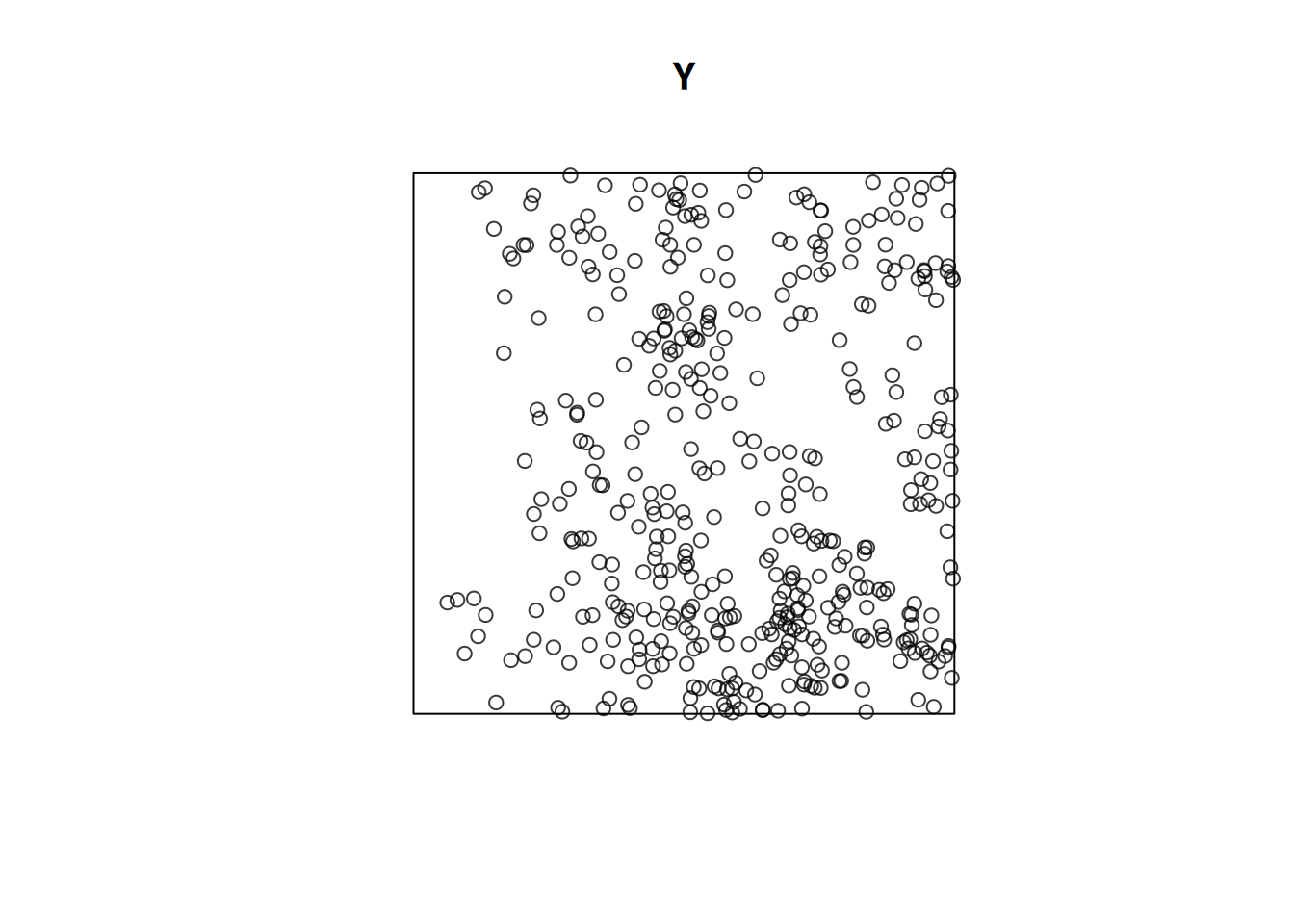
# = min (1, 136, 485, 155000, 21.3)kppm(Y, ~x) |> summary()
# Inhomogeneous cluster point process model
# Fitted to point pattern dataset 'Y'
# Fitted by minimum contrast
# Summary statistic: inhomogeneous K-function
# Minimum contrast fit (object of class "minconfit")
# Model: Thomas process
# Fitted by matching theoretical K function to Y
#
# Internal parameters fitted by minimum contrast ($par):
# kappa sigma2
# 22.69515 0.00808
#
# Fitted cluster parameters:
# kappa scale
# 22.6951 0.0899
# Mean cluster size: [pixel image]
#
# Converged successfully after 93 function evaluations
#
# Starting values of parameters:
# kappa sigma2
# 4.41e+02 1.84e-03
# Domain of integration: [ 0 , 0.25 ]
# Exponents: p= 2, q= 0.25
#
# ----------- TREND -----
# Point process model
# Fitted to data: X
# Fitting method: maximum likelihood (Berman-Turner approximation)
# Model was fitted using glm()
# Algorithm converged
# Call:
# ppm.ppp(Q = X, trend = trend, rename.intercept = FALSE, covariates = covariates,
# covfunargs = covfunargs, use.gam = use.gam, forcefit = TRUE,
# improve.type = ppm.improve.type, improve.args = ppm.improve.args,
# nd = nd, eps = eps)
# Edge correction: "border"
# [border correction distance r = 0 ]
# --------------------------------------------------------------------
# Quadrature scheme (Berman-Turner) = data + dummy + weights
#
# Data pattern:
# Planar point pattern: 441 points
# Average intensity 441 points per square unit
# Window: rectangle = [0, 1] x [0, 1] units
# Window area = 1 square unit
#
# Dummy quadrature points:
# 50 x 50 grid of dummy points, plus 4 corner points
# dummy spacing: 0.02 units
#
# Original dummy parameters: =
# Planar point pattern: 2504 points
# Average intensity 2500 points per square unit
# Window: rectangle = [0, 1] x [0, 1] units
# Window area = 1 square unit
# Quadrature weights:
# (counting weights based on 50 x 50 array of rectangular tiles)
# All weights:
# range: [8e-05, 4e-04] total: 1
# Weights on data points:
# range: [8e-05, 2e-04] total: 0.0803
# Weights on dummy points:
# range: [8e-05, 4e-04] total: 0.92
# --------------------------------------------------------------------
# FITTED :
#
# Nonstationary Poisson process
#
# ---- Intensity: ----
#
# Log intensity: ~x
#
# Fitted trend coefficients:
# (Intercept) x
# 5.35 1.33
#
# Estimate S.E. CI95.lo CI95.hi Ztest Zval
# (Intercept) 5.35 0.115 5.123 5.57 *** 46.48
# x 1.33 0.172 0.997 1.67 *** 7.75
#
# ----------- gory details -----
#
# Fitted regular parameters (theta):
# (Intercept) x
# 5.35 1.33
#
# Fitted exp(theta):
# (Intercept) x
# 210.3 3.8
#
# ----------- CLUSTER -----------
# Model: Thomas process
#
# Fitted cluster parameters:
# kappa scale
# 22.6951 0.0899
# Mean cluster size: [pixel image]
#
# Final standard error and CI
# (allowing for correlation of cluster process):
# Estimate S.E. CI95.lo CI95.hi Ztest Zval
# (Intercept) 5.35 0.382 4.600 6.10 *** 14.01
# x 1.33 0.619 0.121 2.55 * 2.15
#
# ----------- cluster strength indices ----------
# Mean sibling probability 0.303
# Count overdispersion index (on original window): 18.4
# Cluster strength: 0.434
#
# Spatial persistence index (over window): 0
#
# Bound on distance from Poisson process (over window): 1
# = min (1, 882, 93000, 2.1e+07, 291)MaxEnt and species distribution modelling
MaxEnt is a popular software for species distribution modelling in ecology. MaxEnt fits an inhomogeneous Poisson process
Starting from presence (only) observations, it
- adds background (absence) points, uniformly in space
- fits logistic regression models to the 0/1 data, using environmental covariates
- ignores spatial interactions, spatial distances
R package maxnet does that using glmnet (lasso or elasticnet regularization on)
A maxnet example using stars is available in the development version, which can be installed directly from github by remotes::install_github("mrmaxent/maxnet") ; and the same maxnet example using terra (thanks to Ben Tupper).
Relevant papers:
- a paper detailing the equivalence and differences between point pattern models and MaxEnt is found here.
- A statistical explanation of MaxEnt for Ecologists
fitting densities, simulating point patterns
(see day 3 materials)
4.2 geostatistics
kriging interpolation
library(sf)
# Linking to GEOS 3.12.1, GDAL 3.8.4, PROJ 9.4.0; sf_use_s2() is TRUE
no2 <- read.csv(system.file("external/no2.csv",
    package = "gstat"))
crs <- st_crs("EPSG:32632") # a csv doesn't carry a CRS!
st_as_sf(no2, crs = "OGC:CRS84", coords =
    c("station_longitude_deg", "station_latitude_deg")) |>
    st_transform(crs) -> no2.sf
Fit a variogram model:
# The sample variogram:
library(gstat)
#
# Attaching package: 'gstat'
# The following object is masked from 'package:spatstat.explore':
#
#     idw
v = variogram(NO2~1, no2.sf)
v.fit = fit.variogram(v, vgm(1, "Exp", 50000))
plot(v, v.fit)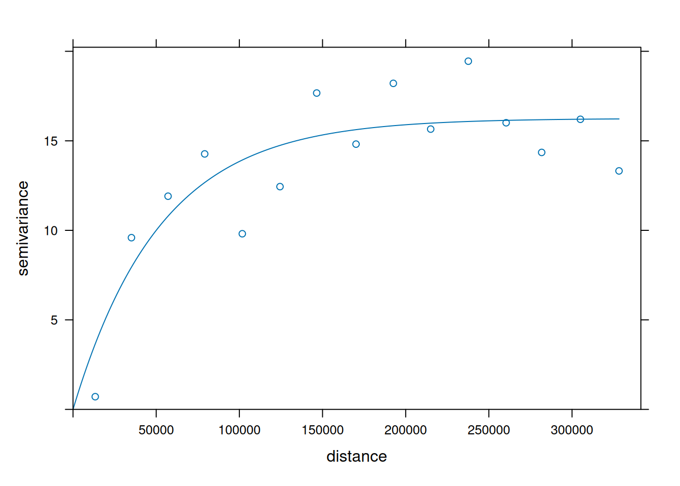
set up a prediction template:
"https://github.com/edzer/sdsr/raw/main/data/de_nuts1.gpkg" |>
  read_sf() |>
  st_transform(crs) -> de
library(stars)
# Loading required package: abind
g2 = st_as_stars(st_bbox(de))
g3 = st_crop(g2, de)
IDW
i = idw(NO2~1, no2.sf, g3)
# [inverse distance weighted interpolation]
BLUP/Kriging
Given this model, we can interpolate using the best unbiased linear predictor (BLUP), also called kriging predictor. Under the model \(Z(s)=m+e(s)\) it estimates \(m\) using generalized least squares, and predicts \(e(s)\) using a weighted mean, where weights are chosen such that \(Var(Z(s_0)-\hat{Z}(s_0))\) is minimized.
k = krige(NO2~1, no2.sf, g3, v.fit)
# [using ordinary kriging]
k$idw = i$var1.pred
k$kriging = k$var1.pred
hook = function() {
  plot(st_geometry(no2.sf), add = TRUE, col = 'yellow')
  plot(st_cast(st_geometry(de), "MULTILINESTRING"), add = TRUE, col = 'red')
}
plot(merge(k[c("kriging", "idw")]), hook = hook, breaks = "equal")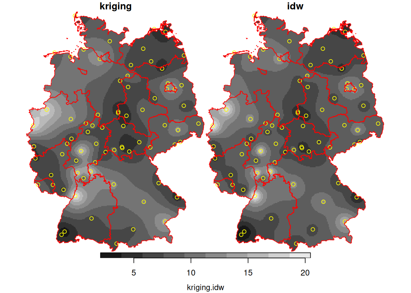
4.3 Kriging with a non-constant mean
Under the model \(Z(s) = X(s)\beta + e(s)\), \(\beta\) is estimated using generalized least squares, and the variogram of regression residuals is needed; see SDS Ch 12.7.
4.4 Conditional simulation
Simulating spatially correlated data
Using a coarse grid, with base R, using the Choleski decomposition algorithm:
set.seed(13579)
g2c = st_as_stars(st_bbox(de), dx = 15000)
g3c = st_crop(g2c, de)
p = st_as_sf(g3c, as_points = TRUE)
d = st_distance(p)
Sigma = variogramLine(v.fit, covariance = TRUE, dist_vector = d)
n = 100
ch = chol(Sigma)
sim = matrix(rnorm(n * nrow(ch)), nrow = n) %*% ch + mean(no2.sf$NO2)
for (i in seq_len(n)) {
    m = g3c[[1]]
    m[!is.na(m)] = sim[i,]
    g3c[[ paste0("sim", i) ]] = m
}
plot(merge(g3c[2:11]), breaks = "equal")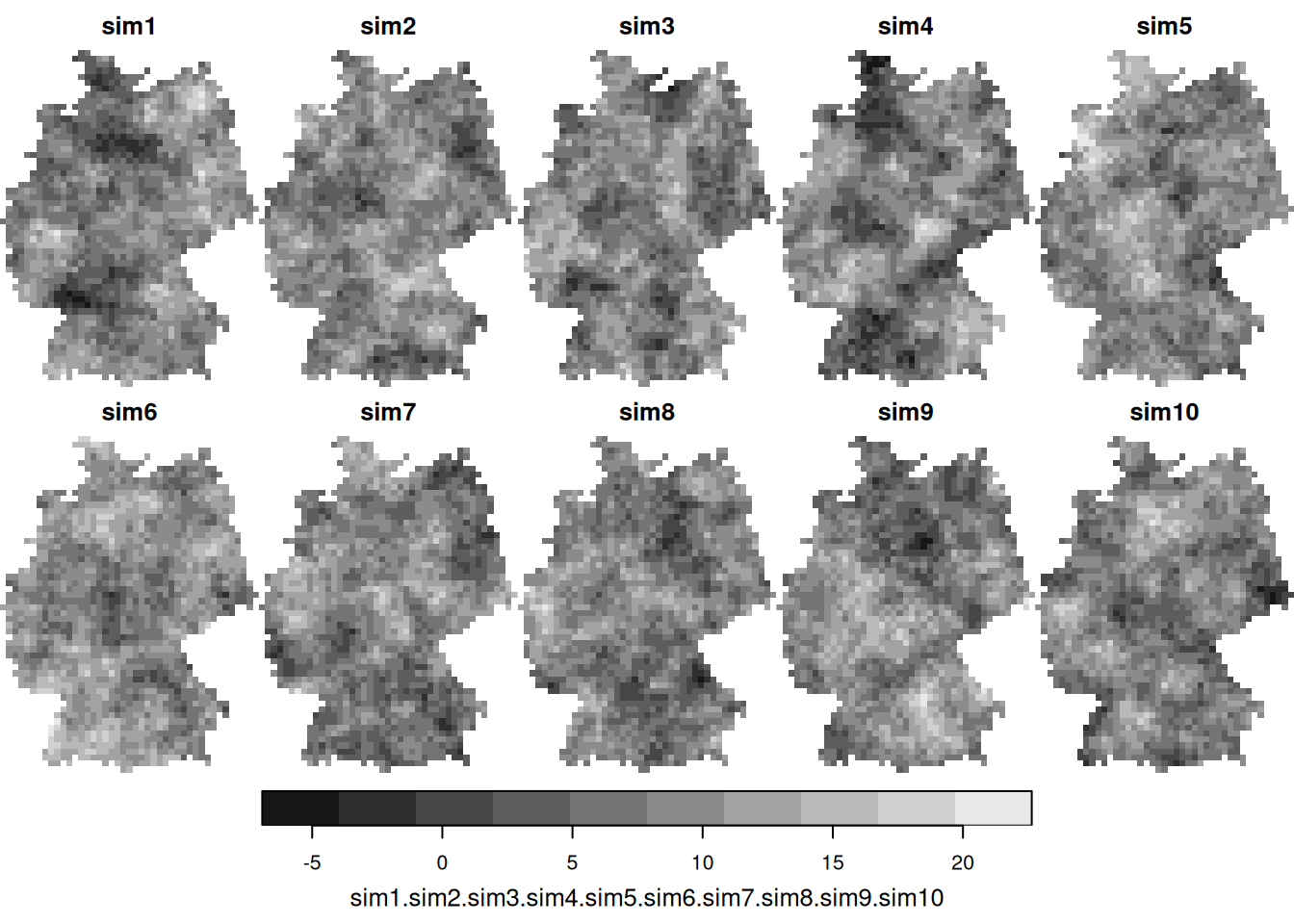
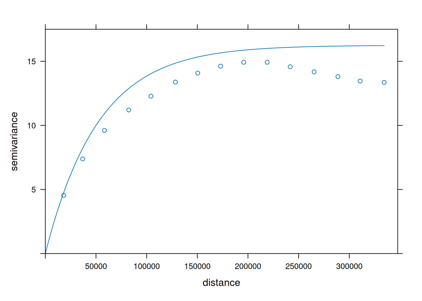
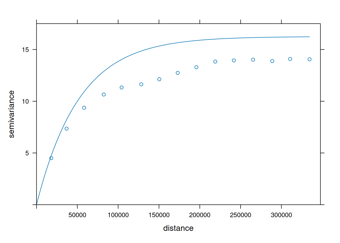
As a check, we could compute the variogram of some of the realisations:
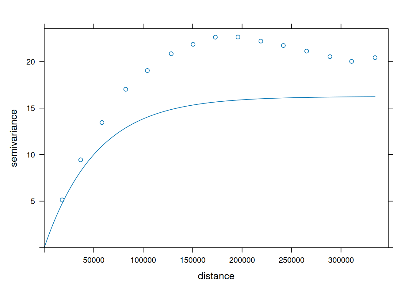
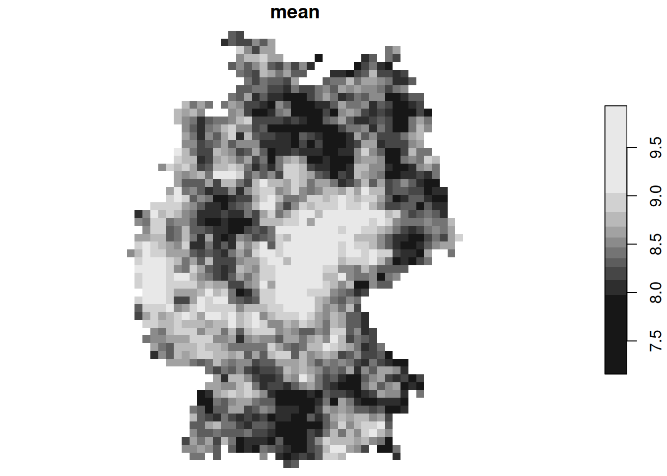
The mean of these simulations is constant, not related to measured values:
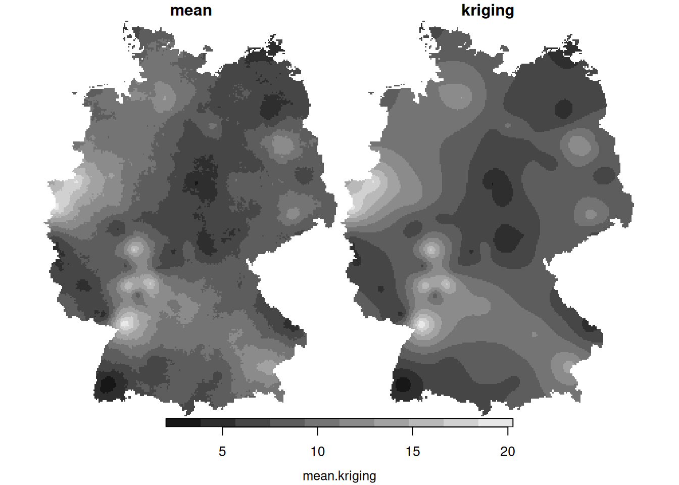
Conditioning simulations on measured values can be done with gstat, using conditional simulation
cs = krige(NO2~1, no2.sf, g3, v.fit, nsim = 50, nmax = 30)
# drawing 50 GLS realisations of beta...
# [using conditional Gaussian simulation]
plot(cs[,,,1:10])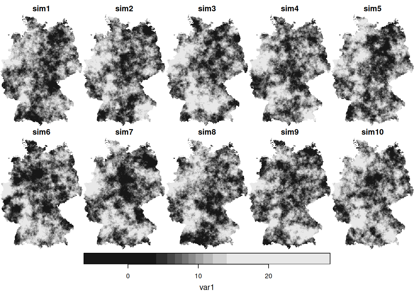
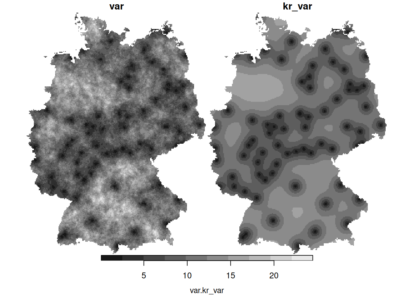
We see that these simulations are much more alike; also their mean and variance resemble that of the kriging mean and variance:
4.5 Exercises
- Try fitting homogeneous Poisson, inhomogeneous Poisson and clustered point process models to the hardcore pattern simulated on day 3.
- Using
krige.cv, carry out a leave-one-out cross validation using the four fitted variogram models of day 3, and compute the root mean square prediction error for all four models. Which one is favourable in this respect? - What causes the differences between the mean and the variance of the conditional simulations (left) and the mean and variance obtained by kriging (right)?
- When comparing (above) the sample variogram of simulated fields with the variogram model used to simulate them, where do you see differences? Can you explain why these are not identical, or hypothesize under which circumstances these would become more similar (or identical)?
- Under which practical data analysis problem would conditional simulations be more useful than the kriging prediction and kriging variance maps?