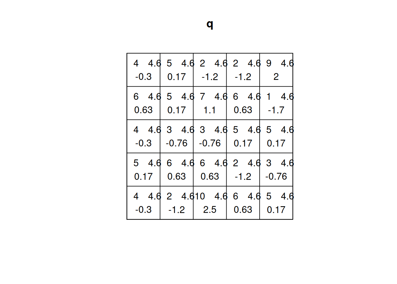
(q=quadrat.test(CSR))# Warning: Some expected counts are small; chi^2 approximation may be# inaccurate# # Chi-squared test of CSR using quadrat counts# # data: CSR# X2 = 25, df = 24, p-value = 0.9# alternative hypothesis: two.sided# # Quadrats: 5 by 5 grid of tilesplot(q)
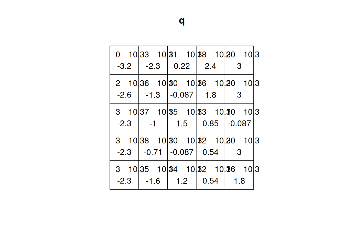
(q=quadrat.test(ppi))# # Chi-squared test of CSR using quadrat counts# # data: ppi# X2 = 88, df = 24, p-value = 6e-09# alternative hypothesis: two.sided# # Quadrats: 5 by 5 grid of tilesplot(q)
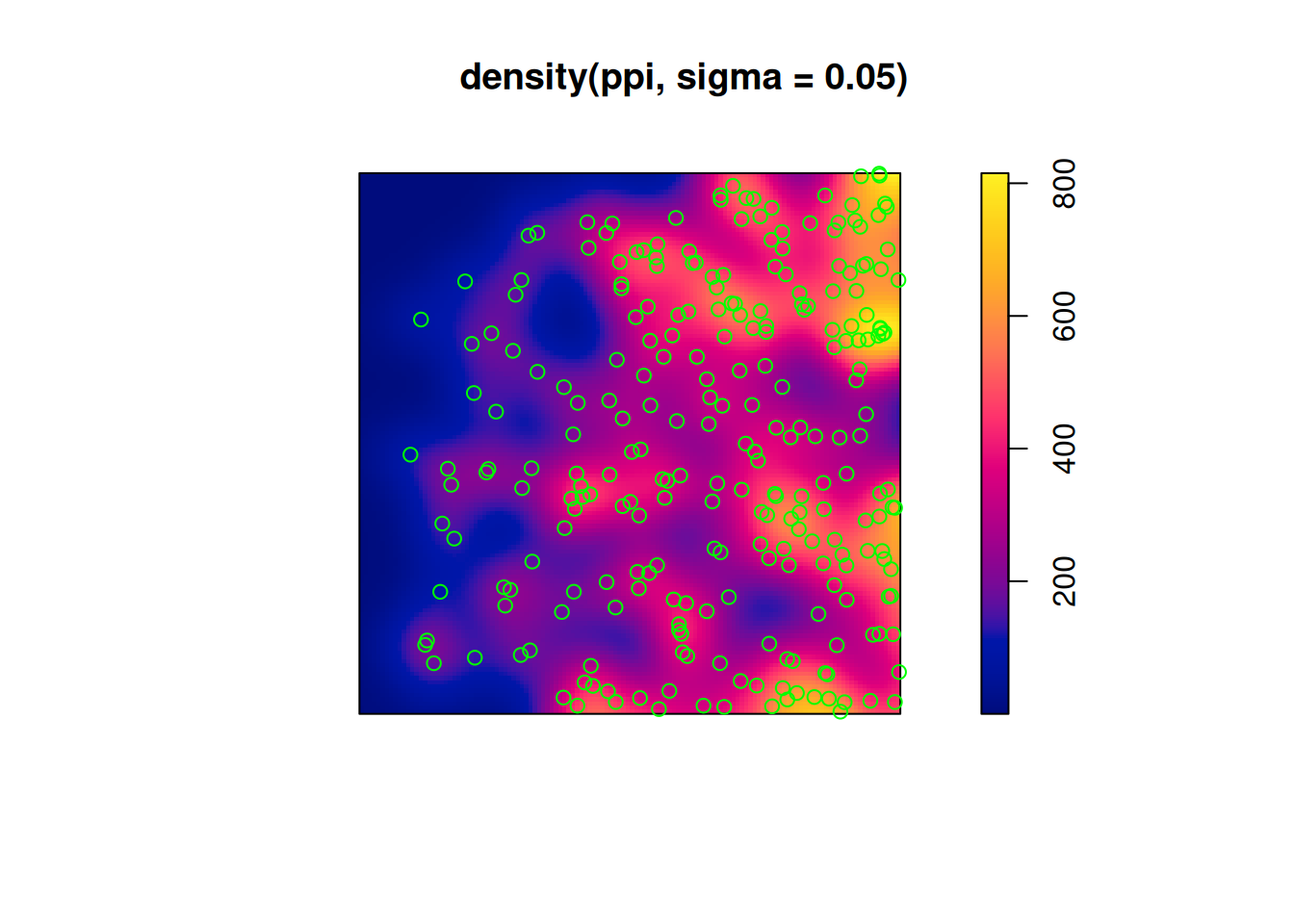
Estimating density
main parameter: bandwidth (sigma): determines the amound of smoothing.
if sigma is not specified: uses bw.diggle, an automatically tuned bandwidth
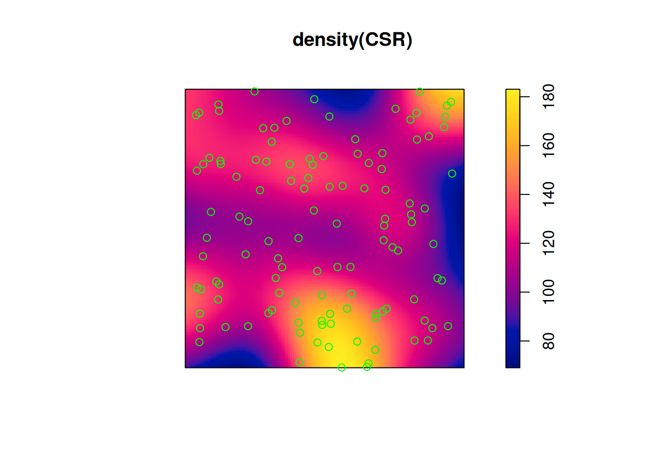
density(ppi, sigma =.05)|>plot()plot(ppi, add =TRUE, col ='green')
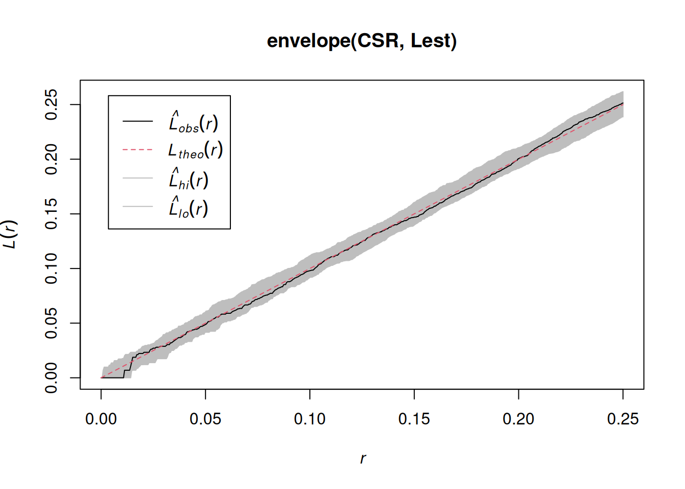
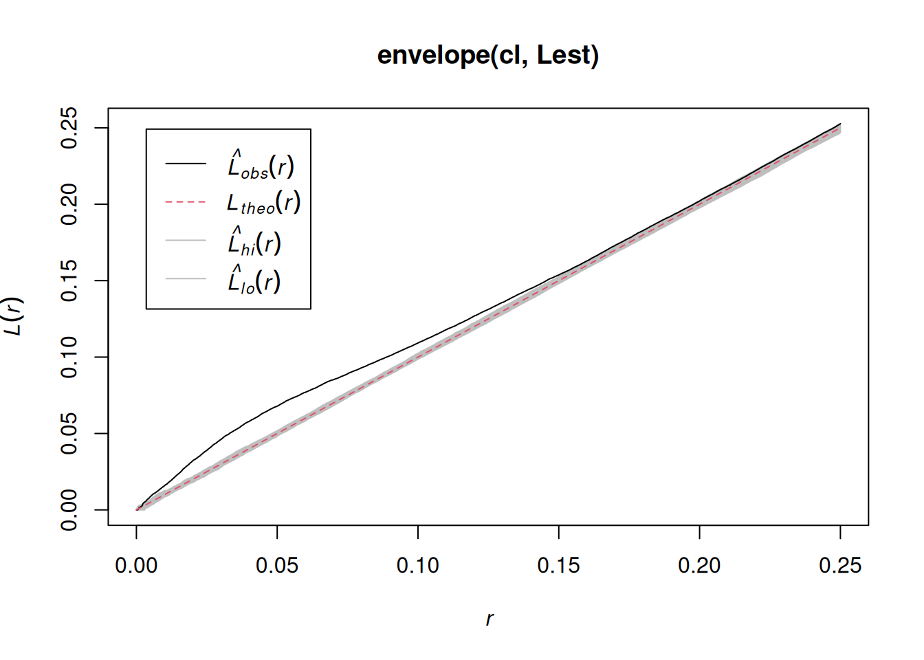
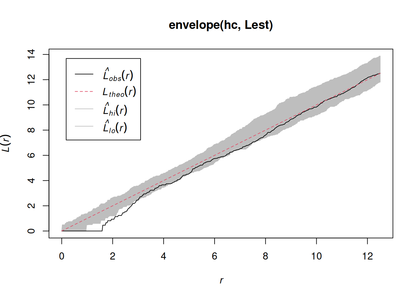
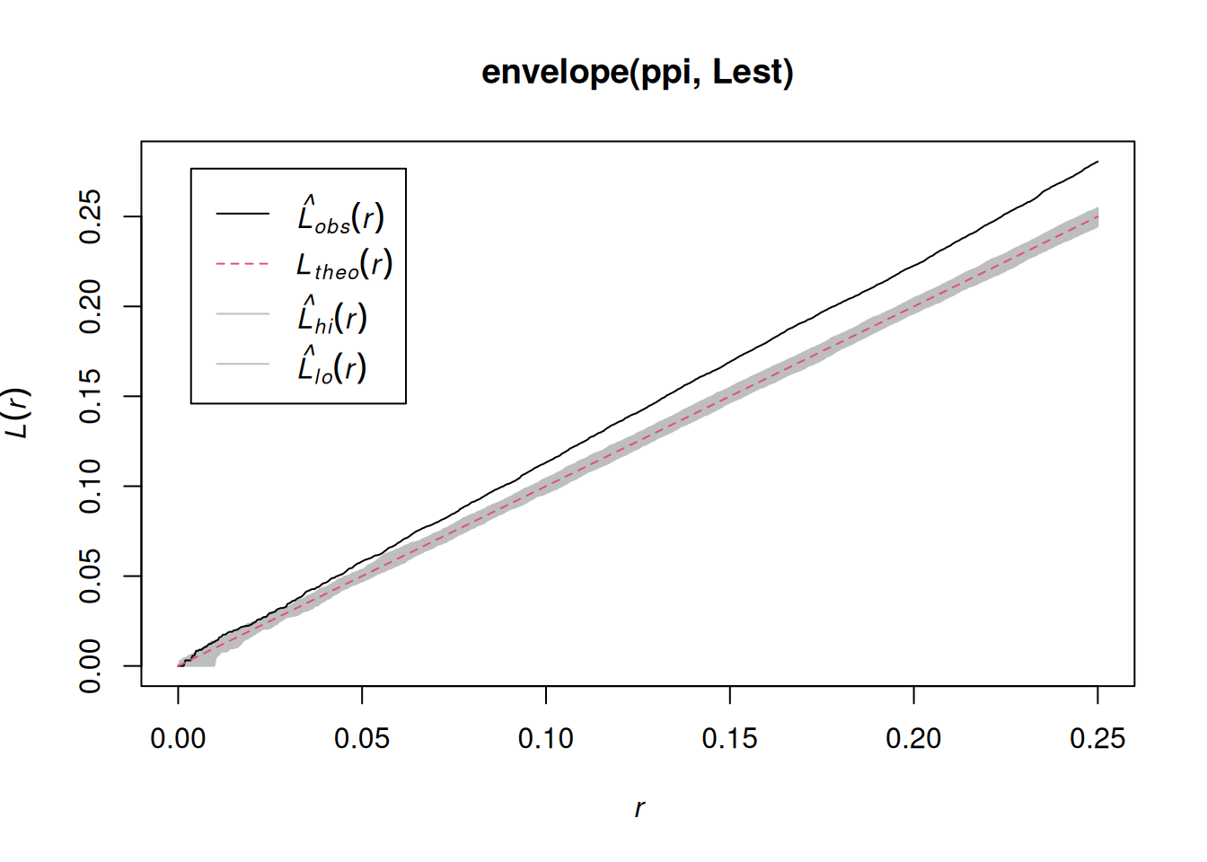
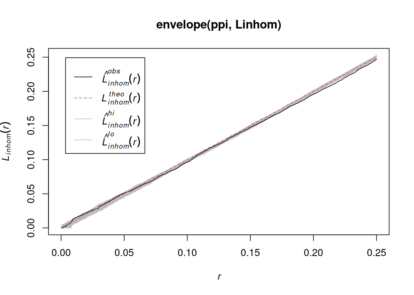
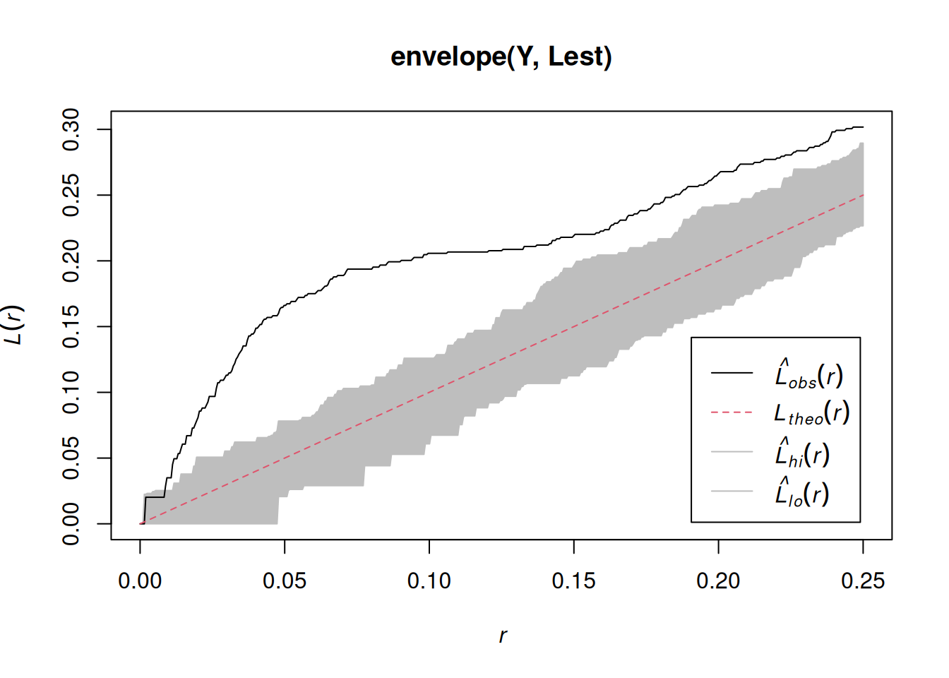
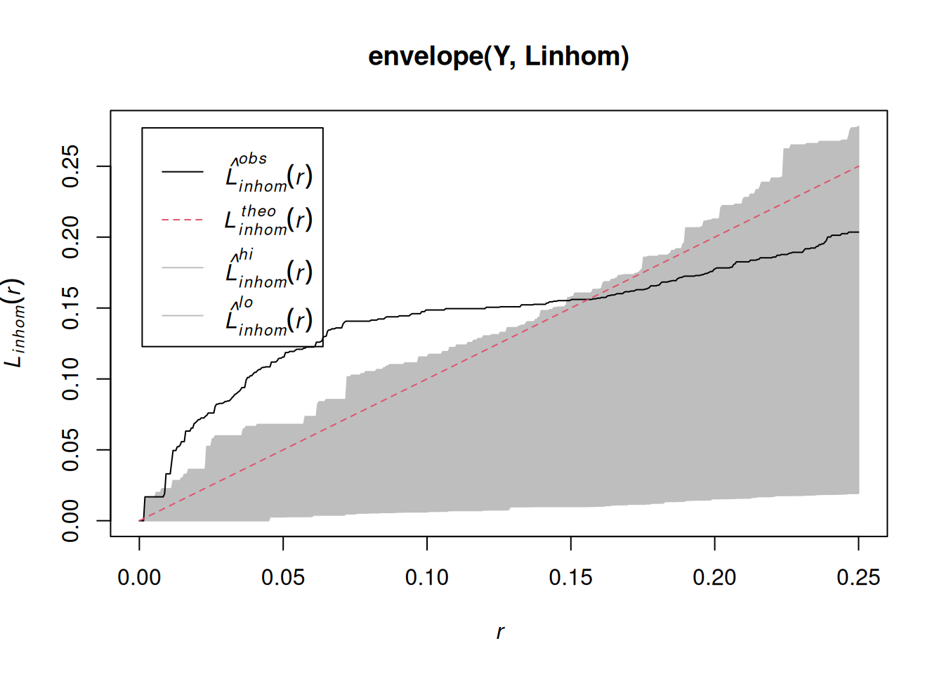
Assessing interactions: clustering/inhibition
The K-function (“Ripley’s K”) is the expected number of additional random (CSR) points within a distance r of a typical random point in the observation window.
The G-function (nearest neighbour distance distribution) is the cumulative distribution function G of the distance from a typical random point of X to the nearest other point of X.
R package gstat was written in 2002/3, from a stand-alone C program that was released under the GPL in 1997. It implements “basic” geostatistical functions for modelling spatial dependence (variograms), kriging interpolation and conditional simulation. It can be used for multivariable kriging (cokriging), as well as for spatiotemporal variography and kriging. Recent updates included support for sf and stars objects.
What are geostatistical data?
Recall from day 1: locations + measured values
The value of interest is measured at a set of sample locations
At other location, this value exists but is missing
The interest is in estimating (predicting) this missing value (interpolation)
The actual sample locations are not of (primary) interest, the signal is in the measured values
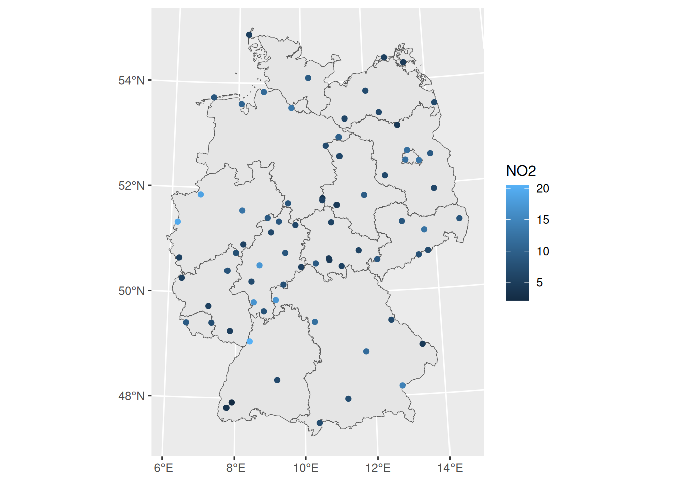
library(sf)# Linking to GEOS 3.12.1, GDAL 3.8.4, PROJ 9.4.0; sf_use_s2() is TRUEno2<-read.csv(system.file("external/no2.csv", package ="gstat"))crs<-st_crs("EPSG:32632")# a csv doesn't carry a CRS!st_as_sf(no2, crs ="OGC:CRS84", coords =c("station_longitude_deg", "station_latitude_deg"))|>st_transform(crs)->no2.sflibrary(ggplot2)# plot(st_geometry(no2.sf))"https://github.com/edzer/sdsr/raw/main/data/de_nuts1.gpkg"|>read_sf()|>st_transform(crs)->deggplot()+geom_sf(data =de)+geom_sf(data =no2.sf, mapping =aes(col =NO2))
Spatial correlation
Lagged scatterplots
“by hand”, base R:
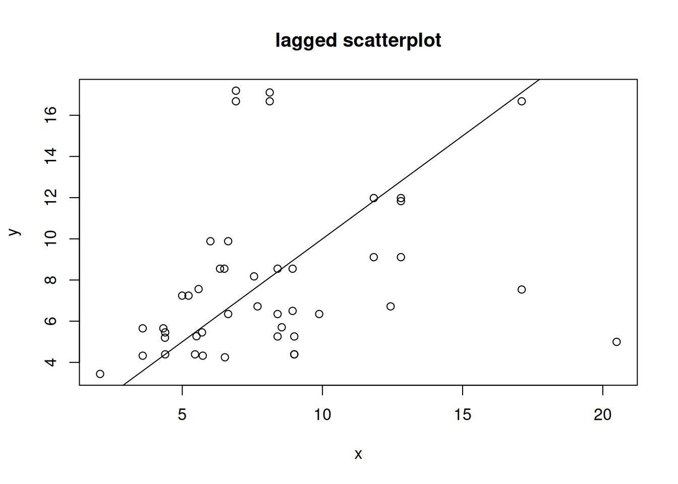
(w=st_is_within_distance(no2.sf, no2.sf, units::set_units(50, km), retain_unique =TRUE))# Sparse geometry binary predicate list of length 74, where# the predicate was `is_within_distance', with retain_unique =# TRUE# first 10 elements:# 1: (empty)# 2: (empty)# 3: 4, 5, 26# 4: 5, 26# 5: (empty)# 6: 30, 72# 7: (empty)# 8: (empty)# 9: (empty)# 10: (empty)d=as.data.frame(w)x=no2.sf$NO2[d$row.id]y=no2.sf$NO2[d$col.id]cor(x, y)# [1] 0.296plot(x, y, main ="lagged scatterplot")abline(0, 1)
using gstat:
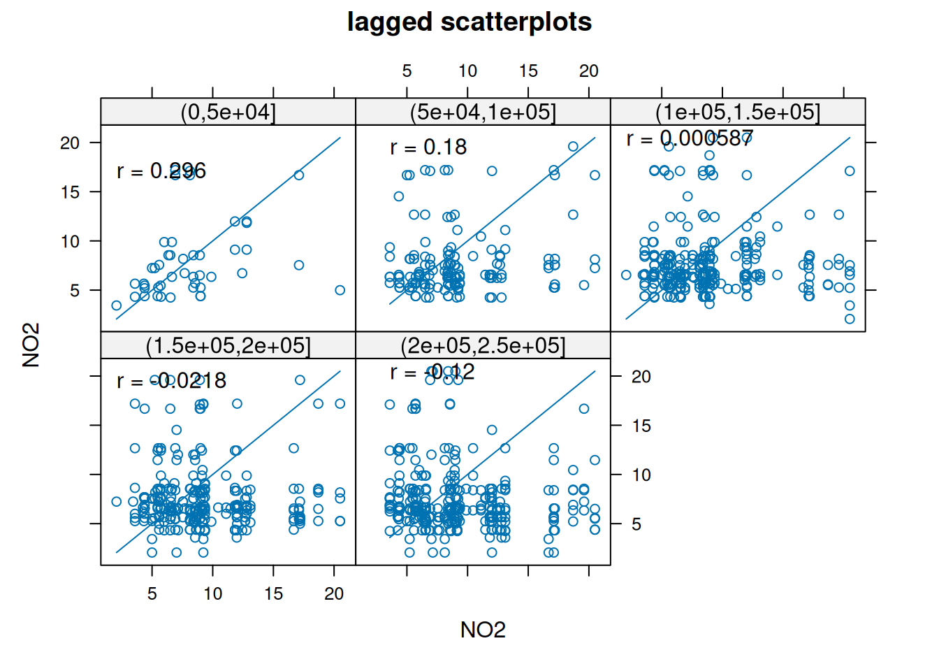
library(gstat)# # Attaching package: 'gstat'# The following object is masked from 'package:spatstat.explore':# # idwhscat(NO2~1, no2.sf, breaks =c(0,50,100,150,200,250)*1000)
Variogram
When we assume \(Z(s)\) has a constant and unknown mean, the spatial dependence can be described by the variogram, defined as \(\gamma(h)
= 0.5 E(Z(s)-Z(s+h))^2\). If the random process \(Z(s)\) has a finite variance, then the variogram is related to the covariance function \(C(h)\) by \(\gamma(h) = C(0)-C(h)\).
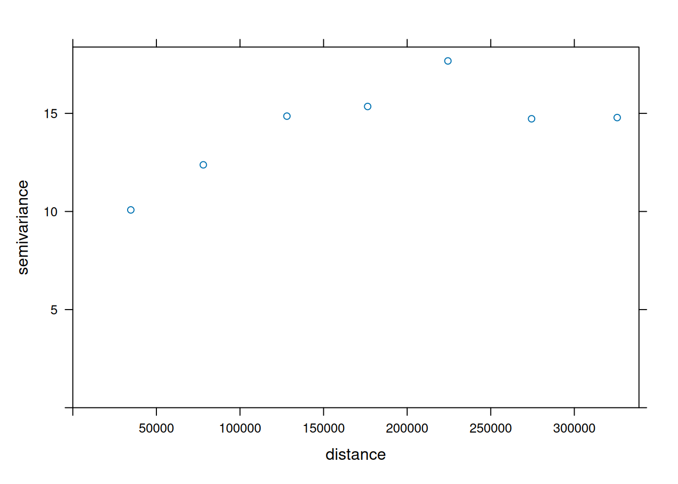
The variogram can be estimated from sample data by averaging squared differences: \[\hat{\gamma}(\tilde{h})=\frac{1}{2N_h}\sum_{i=1}^{N_h}(Z(s_i)-Z(s_i+h))^2 \ \
h \in \tilde{h}\]
divide by \(2N_h\):
if finite, \(\gamma(\infty)=\sigma^2=C(0)\)
semi variance
if data are not gridded, group \(N_h\) pairs \(s_i,s_i+h\) for which \(h \in \tilde{h}\), \(\tilde{h}=[h_1,h_2]\)
rule-of-thumb: choose about 10-25 distance intervals \(\tilde{h}\), from length 0 to about on third of the area size
plot \(\gamma\) against \(\tilde{h}\) taken as the average value of all \(h \in \tilde{h}\)
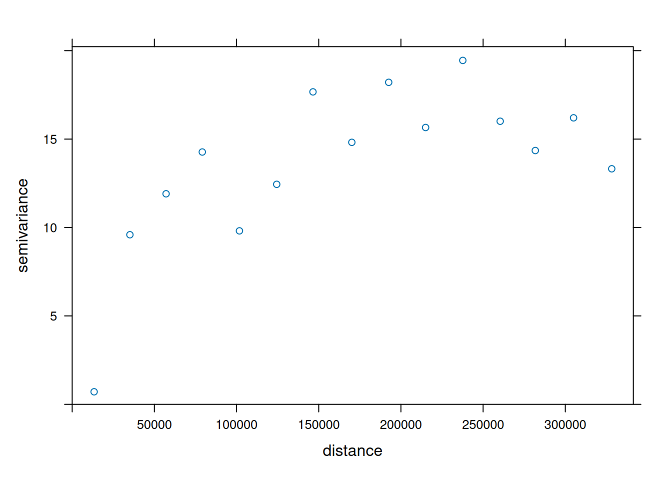
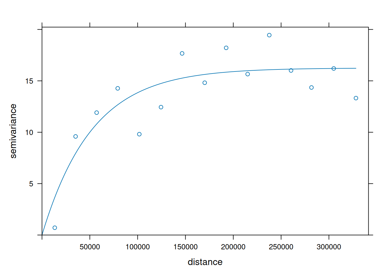
We can compute a variogram “by hand”, using base R:
First, we will consider polygons in relationship to their direct neighbours
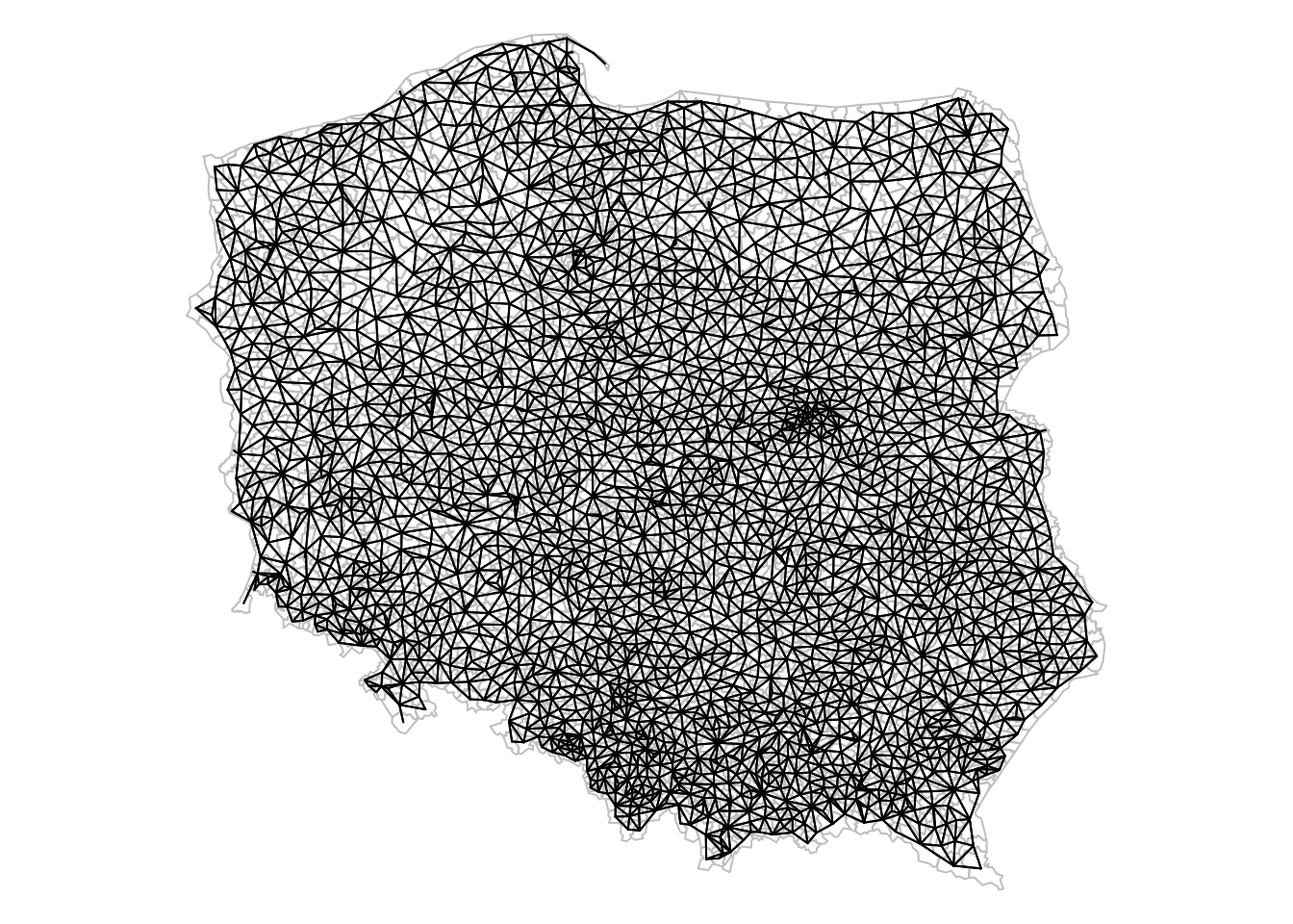
library(spdep)# Loading required package: spDatapol_pres15|>poly2nb(queen =TRUE)->nb_qnb_q# Neighbour list object:# Number of regions: 2495 # Number of nonzero links: 14242 # Percentage nonzero weights: 0.229 # Average number of links: 5.71
Alternative approaches to form neighbourhood matrices:
based on distance, e.g. setting a distance threshold or selecting a fixed number of nearest neighbours
based on triangulating points, for instance polygon centroids
sphere of influence, a modification of triangulation
include neighbours from neighbours
Weights matrices
Weight matrices are needed in analysis, they determine how observations (or residuals) are weighted in a regression model.
(nb_q|>nb2listw(style ="B")->lw_q_B)# Characteristics of weights list object:# Neighbour list object:# Number of regions: 2495 # Number of nonzero links: 14242 # Percentage nonzero weights: 0.229 # Average number of links: 5.71 # # Weights style: B # Weights constants summary:# n nn S0 S1 S2# B 2495 6225025 14242 28484 357280
Spatial correlation: Moran’s I
Moran’s I is defined as
\[
I = \frac{n \sum_{(2)} w_{ij} z_i z_j}{S_0 \sum_{i=1}^{n} z_i^2}
\] where \(x_i, i=1, \ldots, n\) are \(n\) observations on the numeric variable of interest, \(z_i = x_i - \bar{x}\), \(\bar{x} = \sum_{i=1}^{n} x_i / n\), \(\sum_{(2)} = \stackrel{\sum_{i=1}^{n} \sum_{j=1}^{n}}{i \neq j}\), \(w_{ij}\) are the spatial weights, and \(S_0 = \sum_{(2)} w_{ij}\).
We can compute it as
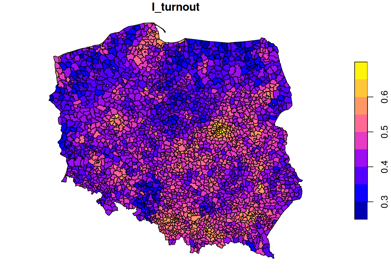
pol_pres15$I_turnout|>moran.test(lw_q_B, randomisation =FALSE, alternative ="two.sided")# # Moran I test under normality# # data: pol_pres15$I_turnout # weights: lw_q_B # # Moran I statistic standard deviate = 58, p-value <2e-16# alternative hypothesis: two.sided# sample estimates:# Moran I statistic Expectation Variance # 0.691434 -0.000401 0.000140plot(pol_pres15["I_turnout"])
A simple linear regression model, assuming independent observations, can be carried out using lm:
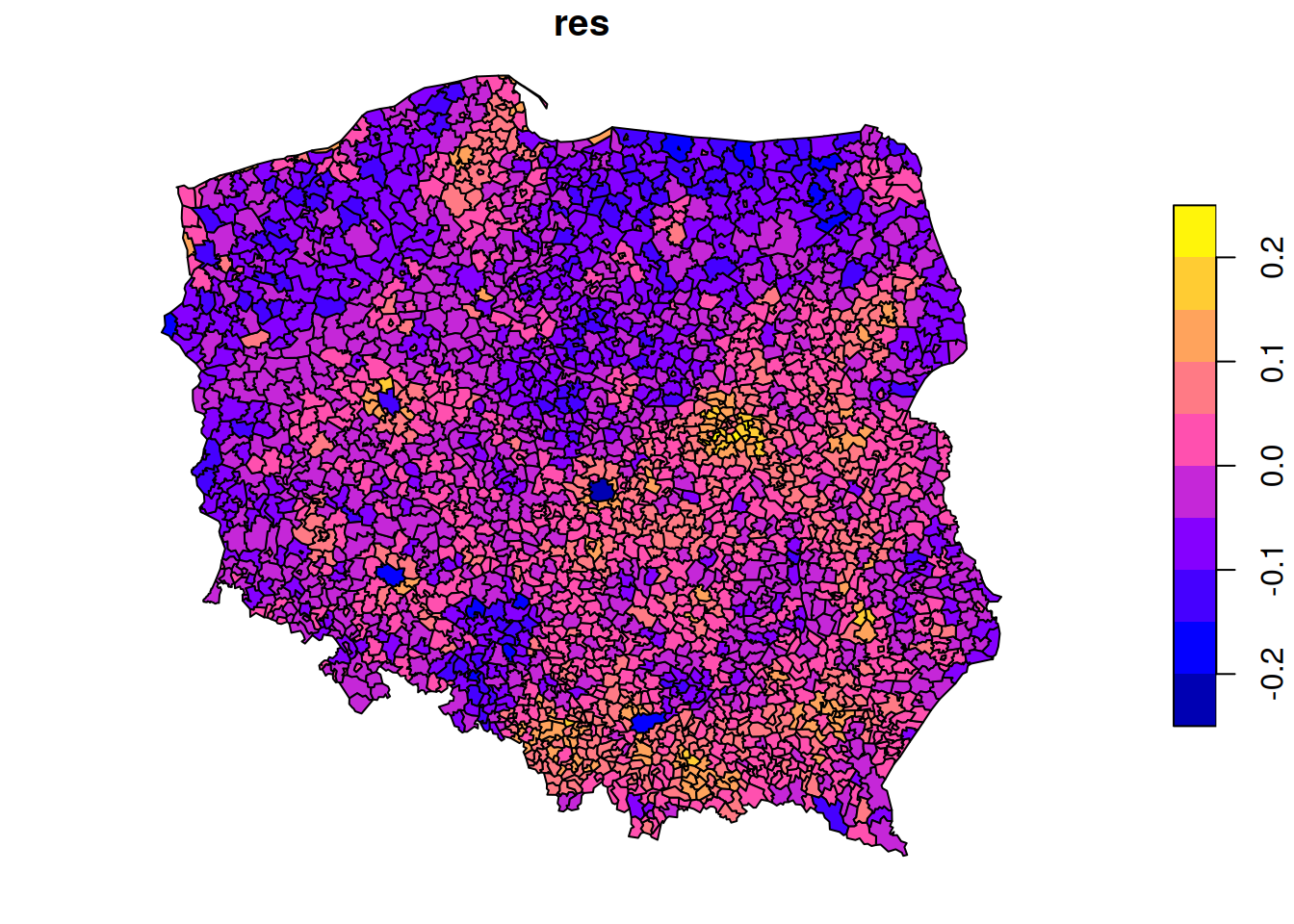
summary(pol_pres15$I_entitled_to_vote)# Min. 1st Qu. Median Mean 3rd Qu. Max. # 1308 4026 6033 12221 10524 594643(lm0<-lm(I_turnout~I_entitled_to_vote, pol_pres15))|>summary()# # Call:# lm(formula = I_turnout ~ I_entitled_to_vote, data = pol_pres15)# # Residuals:# Min 1Q Median 3Q Max # -0.21352 -0.04387 -0.00092 0.04150 0.23611 # # Coefficients:# Estimate Std. Error t value Pr(>|t|) # (Intercept) 4.39e-01 1.34e-03 328.1 <2e-16 ***# I_entitled_to_vote 5.26e-07 4.18e-08 12.6 <2e-16 ***# ---# Signif. codes: 0 '***' 0.001 '**' 0.01 '*' 0.05 '.' 0.1 ' ' 1# # Residual standard error: 0.0618 on 2493 degrees of freedom# Multiple R-squared: 0.0598, Adjusted R-squared: 0.0595 # F-statistic: 159 on 1 and 2493 DF, p-value: <2e-16pol_pres15$res=residuals(lm0)plot(pol_pres15["res"])
A spatial linear regression model (SEM: spatial error model), assuming independent observations, can be carried out using lm:
form=I_turnout~I_entitled_to_votelibrary(spatialreg)# Loading required package: Matrix# # Attaching package: 'spatialreg'# The following objects are masked from 'package:spdep':# # get.ClusterOption, get.coresOption, get.mcOption,# get.VerboseOption, get.ZeroPolicyOption,# set.ClusterOption, set.coresOption, set.mcOption,# set.VerboseOption, set.ZeroPolicyOptionSEM_pres<-errorsarlm(form, data =pol_pres15, Durbin =FALSE, listw =lw_q_B, zero.policy =TRUE)SEM_pres|>summary()# # Call:errorsarlm(formula = form, data = pol_pres15, listw = lw_q_B, # Durbin = FALSE, zero.policy = TRUE)# # Residuals:# Min 1Q Median 3Q Max # -0.1483326 -0.0266702 -0.0025573 0.0217927 0.1659212 # # Type: error # Coefficients: (asymptotic standard errors) # Estimate Std. Error z value Pr(>|z|)# (Intercept) 4.5887e-01 2.3544e-03 194.8968 < 2.2e-16# I_entitled_to_vote 6.8492e-08 2.5677e-08 2.6675 0.007642# # Lambda: 0.138, LR test value: 1964, p-value: < 2.22e-16# Asymptotic standard error: 0.00205# z-value: 67.3, p-value: < 2.22e-16# Wald statistic: 4527, p-value: < 2.22e-16# # Log likelihood: 4390 for error model# ML residual variance (sigma squared): 0.00147, (sigma: 0.0383)# Number of observations: 2495 # Number of parameters estimated: 4 # AIC: -8771, (AIC for lm: -6809)
3.4 Fitting regression models under spatial correlation
Exercises Point Patterns
From the point pattern of wind turbines shown in section 1.4, download the data as GeoPackage, and read them into R
Read the boundary of Germany using rnaturalearth::ne_countries(scale = "large", country = "Germany")
Create a plot showing both the observation window and the point pattern
Do all observations fall inside the observation window?
Create a ppp object from the points and the window
Test whether the point pattern is homogeneous
Create a plot with the (estimated) density of the wind turbines, with the turbine points added
Verify that the mean density multiplied by the area of the window approximates the number of turbines
Test for interaction: create diagnostic plots to verify whether the point pattern is clustered, or exhibits repulsion
3.5 Exercises Geostat.
Compute the variogram cloud of NO2 using variogram() and argument cloud = TRUE. (a) How does the resulting object differ from the “regular” variogram (use the head command on both objects); (b) what do the “left” and “right” fields refer to? (c) when we plot the resulting variogram cloud object, does it still indicate spatial correlation?
Compute the variogram of NO2 as above, and change the arguments cutoff and width into very large or small values. What do they do?
Fit a spherical model to the sample variogram of NO2, using fit.variogram() (follow the example below, replace “Exp” with “Sph”)
Fit a Matern model (“Mat”) to the sample variogram using different values for kappa (e.g., 0.3 and 4), and plot the resulting models with the sample variogram.
Which model do you like the best? Can the SSErr attribute of the fitted model be used to compare the models? How else can variogram model fits be compared?
3.6 Exercises Lattice data
Compare the results of the simple linear regression with the spatial error model
Compare the maps of residuals of both models
Fit a spatial Durbin error model (SDEM), using Durbin = TRUE in the same call to errorsarlm; compare the output of the Spatial Durbin model with that of the error model.
carry out a likelyhood ratio test to compare the SEM and SDEM models (lmtest::lrtest(), see the SDS book Ch 17)
3.7 Further reading
E. Pebesma, 2018. Simple Features for R: Standardized Support for Spatial Vector Data. The R Journal 10:1, 439-446.
A. Baddeley, E. Rubak and R Turner, 2016. Spatial Point Patterns: methodology and Applications in R; Chapman and Hall/CRC 810 pages.
J. Illian, A. Penttinen, H. Stoyan and D. Stoyan, 2008. Statistical Analysis and Modelling of Spatial Point Patterns; Wiley, 534 pages.
Source Code
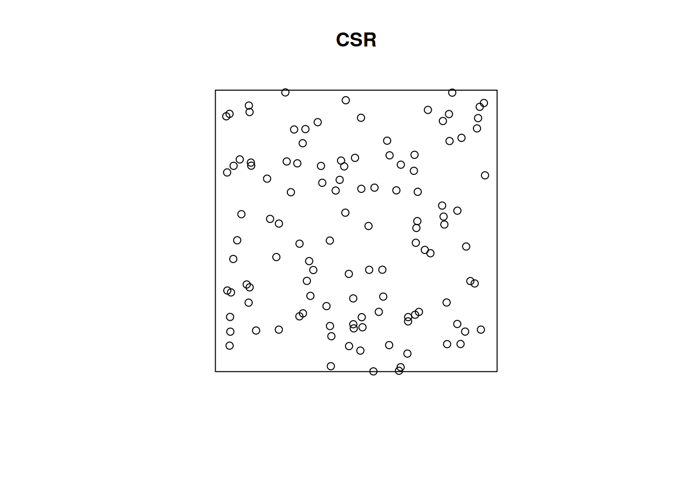
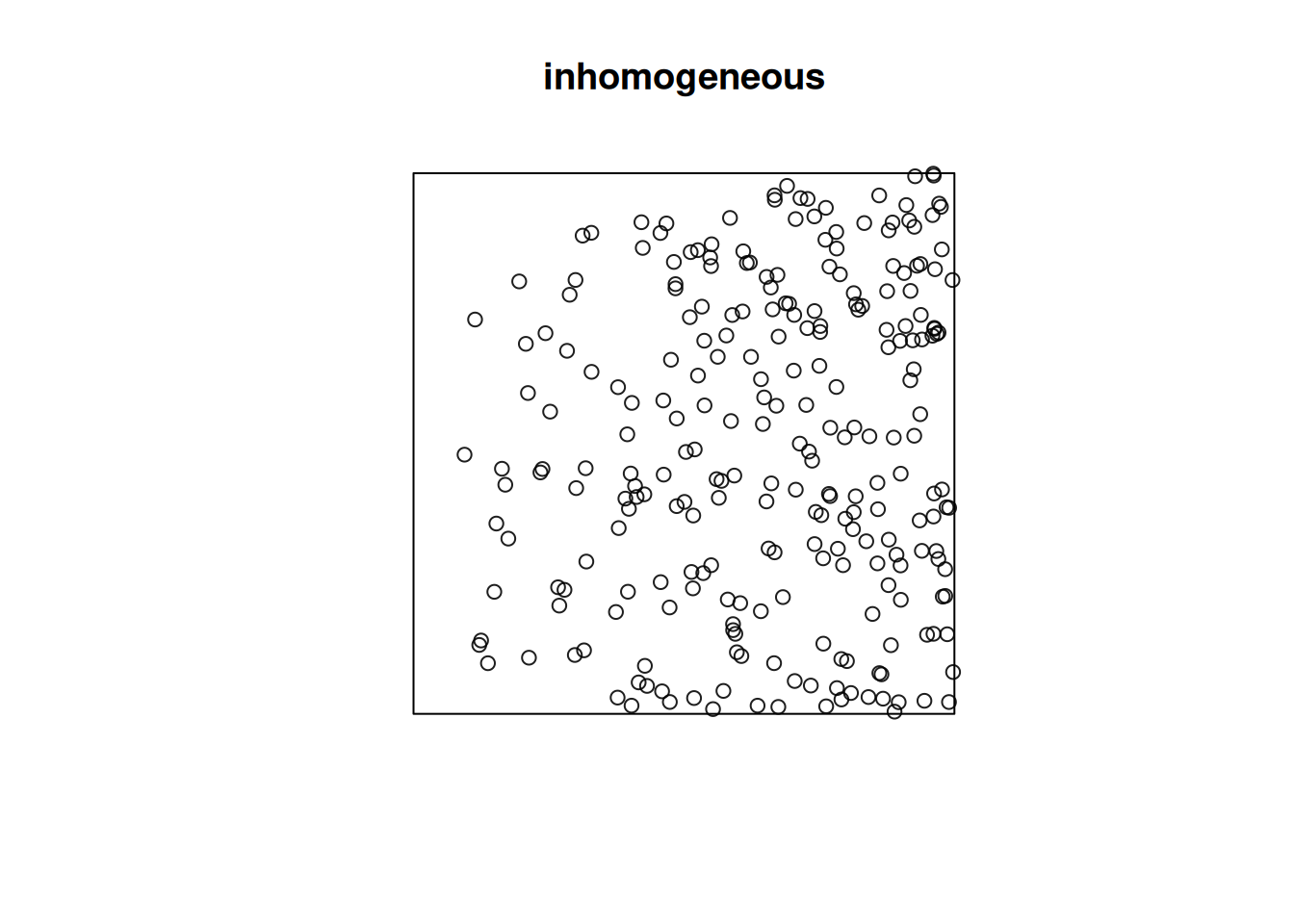
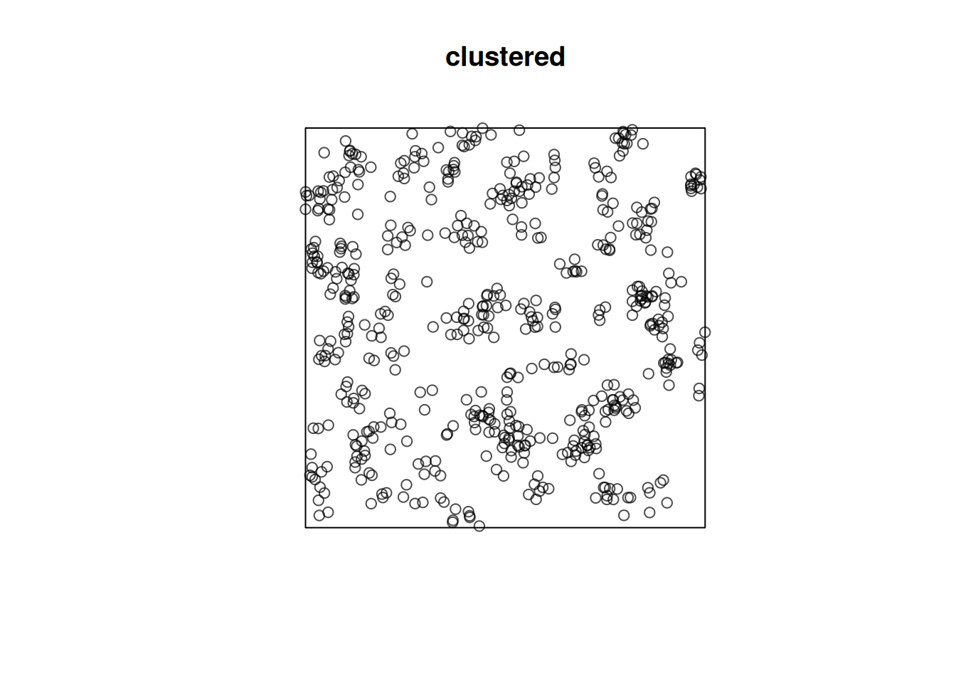
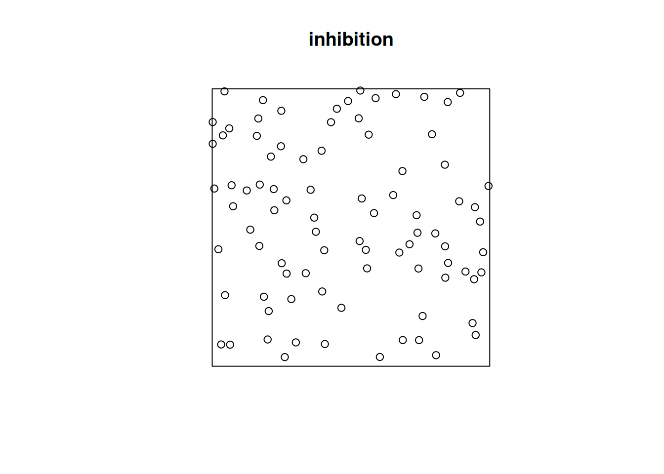
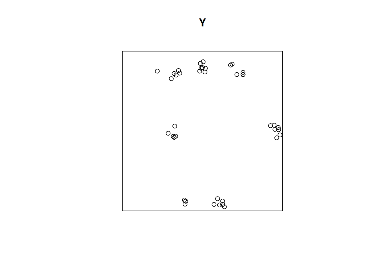
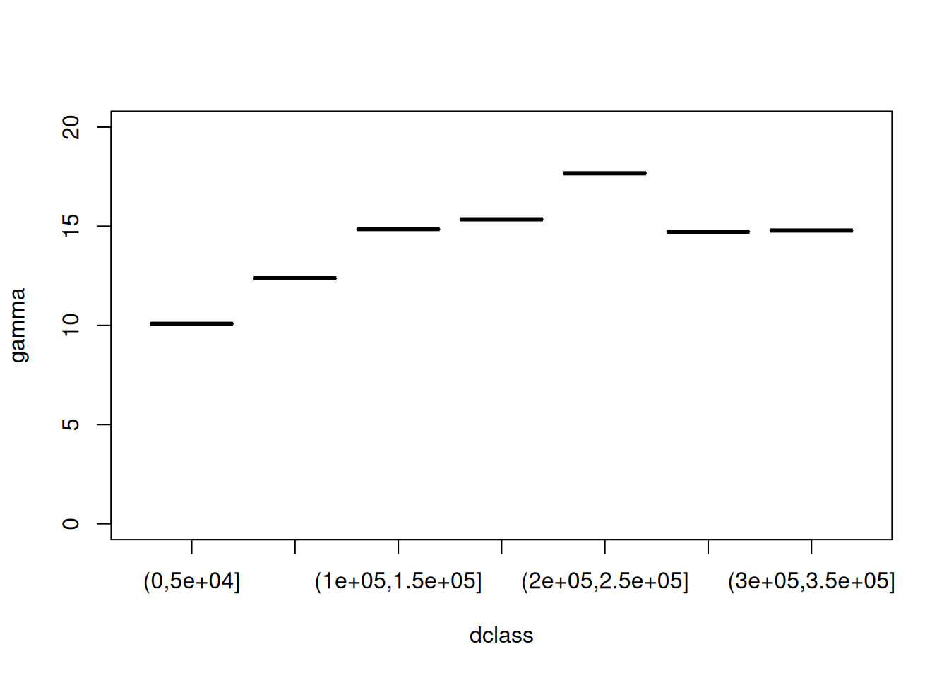
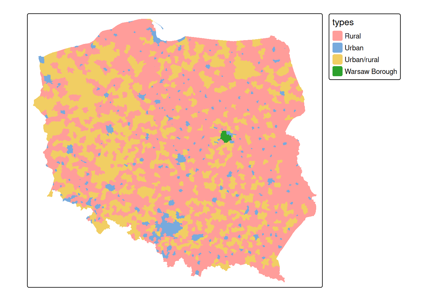
# inference: spatial correlation, fitting models## Spatial correlation for point patterns, ### Intro to `spatstat`Consider a point pattern that consist of- a set of known coordinates- an observation windowWe can ask ourselves: our point **pattern** be a realisation of a *completely spatially random* (CSR) **process**? A CSR process has1. a spatially constant intensity (*mean*: first order property)2. completely independent locations (*interactions*: second order property)e.g.```{r}library(spatstat)set.seed(13431)CSR =rpoispp(100)plot(CSR)```Or does it have a non-constant intensity, but otherwise independent points?```{r}set.seed(1357)ppi =rpoispp(function(x,y,...) 500* x)plot(ppi, main ="inhomogeneous")```Or does it have constant intensity, but dependent points:```{r}cl <-rThomas(100, .02, 5)plot(cl, main ="clustered")``````{r}hc <-rHardcore(0.05,1.5,square(50)) plot(hc, main ="inhibition")```or a combination:```{r}#ff <- function(x,y) { 4 * exp(2 * abs(x) - 1) }set.seed(1357)ff <-function(x,y) 10* xZ <-as.im(ff, owin())Y <-rMatClust(10, 0.05, Z)plot(Y)```### Checking homogeneity```{r}(q =quadrat.test(CSR))plot(q)(q =quadrat.test(ppi))plot(q)```### Estimating density- main parameter: bandwidth (`sigma`): determines the amound of smoothing.- if `sigma` is not specified: uses `bw.diggle`, an automatically tuned bandwidthCorrection for `edge` effect?```{r}density(CSR) |>plot()plot(CSR, add =TRUE, col ='green')density(ppi) |>plot()plot(ppi, add =TRUE, col ='green')density(ppi, sigma = .05) |>plot()plot(ppi, add =TRUE, col ='green')```### Assessing interactions: clustering/inhibitionThe K-function ("Ripley's K") is the expected number of additional random (CSR) points within a distance r of a typical random point in the observation window.The G-function (nearest neighbour distance distribution) is the cumulative distribution function G of the distance from a typical random point of X to the nearest other point of X.```{r}envelope(CSR, Lest) |>plot()envelope(cl, Lest) |>plot()envelope(hc, Lest) |>plot()envelope(ppi, Lest) |>plot()envelope(ppi, Linhom) |>plot()envelope(Y , Lest) |>plot()envelope(Y , Linhom) |>plot()```## Spatial correlation for geostatistical data### `gstat`R package `gstat` was written in 2002/3, from a stand-alone C program that was released under the GPL in 1997. It implements "basic" geostatistical functions for modelling spatial dependence (variograms), kriging interpolation and conditional simulation. It can be used for multivariable kriging (cokriging), as well as for spatiotemporal variography and kriging. Recent updates included support for `sf` and `stars` objects.### What are geostatistical data?Recall from day 1: locations + measured values- The value of interest is measured at a set of sample locations- At other location, this value exists but is *missing*- The interest is in estimating (predicting) this missing value (interpolation)- The actual sample locations are not of (primary) interest, the signal is in the measured values```{r}library(sf)no2 <-read.csv(system.file("external/no2.csv",package ="gstat"))crs <-st_crs("EPSG:32632") # a csv doesn't carry a CRS!st_as_sf(no2, crs ="OGC:CRS84", coords =c("station_longitude_deg", "station_latitude_deg")) |>st_transform(crs) -> no2.sflibrary(ggplot2)# plot(st_geometry(no2.sf))"https://github.com/edzer/sdsr/raw/main/data/de_nuts1.gpkg"|>read_sf() |>st_transform(crs) -> deggplot() +geom_sf(data = de) +geom_sf(data = no2.sf, mapping =aes(col = NO2))```### Spatial correlation#### Lagged scatterplots"by hand", base R:```{r}(w =st_is_within_distance(no2.sf, no2.sf, units::set_units(50, km), retain_unique =TRUE))d =as.data.frame(w)x = no2.sf$NO2[d$row.id]y = no2.sf$NO2[d$col.id]cor(x, y)plot(x, y, main ="lagged scatterplot")abline(0, 1)```using gstat:```{r}library(gstat)hscat(NO2~1, no2.sf, breaks =c(0,50,100,150,200,250)*1000)```#### VariogramWhen we assume $Z(s)$ has a constant and unknown mean, the spatial dependence can be described by the variogram, defined as $\gamma(h)= 0.5 E(Z(s)-Z(s+h))^2$. If the random process $Z(s)$ has a finite variance, then the variogram is related to the covariance function $C(h)$ by $\gamma(h) = C(0)-C(h)$.The variogram can be estimated from sample data by averaging squared differences: $$\hat{\gamma}(\tilde{h})=\frac{1}{2N_h}\sum_{i=1}^{N_h}(Z(s_i)-Z(s_i+h))^2 \ \h \in \tilde{h}$$- divide by $2N_h$: - if finite, $\gamma(\infty)=\sigma^2=C(0)$ - *semi* variance- if data are not gridded, group $N_h$ pairs $s_i,s_i+h$ for which $h \in \tilde{h}$, $\tilde{h}=[h_1,h_2]$- rule-of-thumb: choose about 10-25 distance intervals $\tilde{h}$, from length 0 to about on third of the area size- plot $\gamma$ against $\tilde{h}$ taken as the average value of all $h \in \tilde{h}$We can compute a variogram "by hand", using base R:```{r}z = no2.sf$NO2z2 =0.5*outer(z, z, FUN ="-")^2# (Z(s)-Z(s+h))^2d =as.matrix(st_distance(no2.sf)) # hvcloud =data.frame(dist =as.vector(d), gamma =as.vector(z2))vcloud = vcloud[vcloud$dist !=0,]vcloud$dclass =cut(vcloud$dist, c(0, 50, 100, 150, 200, 250, 300, 350) *1000)v =aggregate(gamma~dclass, vcloud, mean)plot(gamma ~ dclass, v, ylim =c(0, 20))```using gstat:```{r}vv =variogram(NO2~1, no2.sf, width =50000, cutoff =350000)vv$gamma - v$gammaplot(vv)```#### Fit a variogram model```{r}# The sample variogram:v =variogram(NO2~1, no2.sf)plot(v)```fit a model, e.g. an exponential model:```{r}v.fit =fit.variogram(v, vgm(1, "Exp", 50000))plot(v, v.fit)```## Spatial correlation in lattice data### Analysing lattice data: neighbours, weights, models```{r}library(sf)data(pol_pres15, package ="spDataLarge")pol_pres15 |>subset(select =c(TERYT, name, types)) |>head()library(tmap, warn.conflicts =FALSE)tm_shape(pol_pres15) +tm_fill("types")```We need to make the geometries valid first,```{r}st_is_valid(pol_pres15) |>all()pol_pres15 <-st_make_valid(pol_pres15)st_is_valid(pol_pres15) |>all()```First, we will consider polygons in relationship to their direct neighbours```{r}library(spdep)pol_pres15 |>poly2nb(queen =TRUE) -> nb_qnb_q```Is the graph connected?```{r}(nb_q |>n.comp.nb())$nc``````{r}par(mar =rep(0, 4))pol_pres15 |>st_geometry() |>st_centroid(of_largest_polygon =TRUE) -> coordsplot(st_geometry(pol_pres15), border ='grey')plot(nb_q, coords = coords, add =TRUE, points =FALSE)```Alternative approaches to form neighbourhood matrices:- based on distance, e.g. setting a distance threshold or selecting a fixed number of nearest neighbours- based on triangulating points, for instance polygon centroids- sphere of influence, a modification of triangulation- include neighbours from neighbours#### Weights matricesWeight matrices are needed in analysis, they determine how observations(or residuals) are weighted in a regression model.```{r}(nb_q |>nb2listw(style ="B") -> lw_q_B)```#### Spatial correlation: Moran's IMoran's I is defined as$$I = \frac{n \sum_{(2)} w_{ij} z_i z_j}{S_0 \sum_{i=1}^{n} z_i^2}$$where $x_i, i=1, \ldots, n$ are $n$ observations on the numeric variable of interest, $z_i = x_i - \bar{x}$, $\bar{x} = \sum_{i=1}^{n} x_i / n$, $\sum_{(2)} = \stackrel{\sum_{i=1}^{n} \sum_{j=1}^{n}}{i \neq j}$, $w_{ij}$ are the spatial weights, and $S_0 = \sum_{(2)} w_{ij}$. We can compute it as```{r}pol_pres15$I_turnout |>moran.test(lw_q_B, randomisation =FALSE,alternative ="two.sided")plot(pol_pres15["I_turnout"])```A simple linear regression model, assuming independent observations, can be carried out using `lm`:```{r}summary(pol_pres15$I_entitled_to_vote)(lm0 <-lm(I_turnout ~ I_entitled_to_vote, pol_pres15)) |>summary()pol_pres15$res =residuals(lm0)plot(pol_pres15["res"])```A spatial linear regression model (SEM: spatial error model),assuming independent observations, can be carried out using `lm`:```{r}form = I_turnout ~ I_entitled_to_votelibrary(spatialreg)SEM_pres <-errorsarlm(form, data = pol_pres15, Durbin =FALSE,listw = lw_q_B, zero.policy =TRUE) SEM_pres |>summary()```## Fitting regression models under spatial correlation### Exercises Point Patterns1. From the point pattern of wind turbines shown in section 1.4, download the data as GeoPackage, and read them into R1. Read the boundary of Germany using `rnaturalearth::ne_countries(scale = "large", country = "Germany")`1. Create a plot showing both the observation window and the point pattern1. Do all observations fall inside the observation window?1. Create a ppp object from the points and the window1. Test whether the point pattern is homogeneous1. Create a plot with the (estimated) density of the wind turbines, with the turbine points added1. Verify that the mean density multiplied by the area of the window approximates the number of turbines1. Test for interaction: create diagnostic plots to verify whether the point pattern is clustered, or exhibits repulsion## Exercises Geostat.1. Compute the variogram cloud of NO2 using `variogram()` and argument `cloud = TRUE`. (a) How does the resulting object differ from the "regular" variogram (use the `head` command on both objects); (b) what do the "left" and "right" fields refer to? (c) when we plot the resulting variogram cloud object, does it still indicate spatial correlation?2. Compute the variogram of NO2 as above, and change the arguments `cutoff` and `width` into very large or small values. What do they do?3. Fit a spherical model to the sample variogram of NO2, using `fit.variogram()` (follow the example below, replace "Exp" with "Sph")4. Fit a Matern model ("Mat") to the sample variogram using different values for kappa (e.g., 0.3 and 4), and plot the resulting models with the sample variogram.5. Which model do you like the best? Can the SSErr attribute of the fitted model be used to compare the models? How else can variogram model fits be compared?## Exercises Lattice data1. Compare the results of the simple linear regression with the spatial error model2. Compare the maps of residuals of both models2. Fit a spatial Durbin error model (SDEM), using `Durbin = TRUE` in the same call to `errorsarlm`; compare the output of the Spatial Durbin model with that of the error model.3. carry out a likelyhood ratio test to compare the SEM and SDEM models (`lmtest::lrtest()`, see the SDS book Ch 17)## Further reading- E. Pebesma, 2018. Simple Features for R: Standardized Support for Spatial Vector Data. The R Journal 10:1, [439-446](https://journal.r-project.org/archive/2018/RJ-2018-009/index.html).- A. Baddeley, E. Rubak and R Turner, 2016. Spatial Point Patterns: methodology and Applications in R; Chapman and Hall/CRC 810 pages.- J. Illian, A. Penttinen, H. Stoyan and D. Stoyan, 2008. Statistical Analysis and Modelling of Spatial Point Patterns; Wiley, 534 pages.