# Data Cubes {#sec-datacube}
\index{data cubes}
\index{array data}
Data cubes arise naturally when we observe properties of a set of
geometries repeatedly over time. Time information may sometimes be
considered as an attribute of a feature, such as when we register the year
of construction of a building or the date of birth of a person
(@sec-featureattributes). In other cases it may refer to the time
of observing an attribute, or the time for which a prediction of an
attribute has been made. In these cases, time is on equal footing
with space, and time and space together describe the physical
dimensions over which we observe, model, predict, or make
forecasts for.
One way of considering our world is that of a four-dimensional
space, with three space dimensions and one time dimension. In that view,
events become "things" or "objects" that have as duration their
size on the time dimension [@galton]. Although such a view does
not align well with how we experience and describe the world,
from a data analytical perspective, four numbers, along with their
reference systems, suffice to describe space and time coordinates
of an observation associated with a point location and time instance.
We define data cubes as array data with one or more array dimensions
associated with space and/or time [@lu2018multidimensional]. This
implies that raster data, features with attributes, and time series
data are all special cases of data cubes. Since we do not restrict
to three-dimensional structures, we actually mean _hypercubes_
rather than cubes, and as the cube extent of the different dimensions
does not have to be identical, or have comparable units, the better
term would be _hyper-rectangle_. For simplicity, we talk about data
cubes instead.
\index{hypercube}
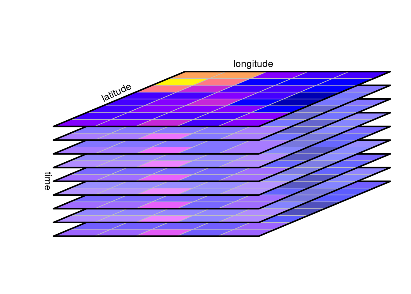
A canonical form of a data cube is shown in @fig-cube:
it shows in a perspective plot a set of raster layers for the same
region that were collected (observed, or modelled) at different time
steps. The three cube dimensions longitude, latitude, and time, are
thought of as being orthogonal. Arbitrary two-dimensional cube
slices are obtained by fixing one of the dimensions at a particular
value, one-dimensional slices are obtained by fixing two of the
dimensions at a particular value, and a scalar is obtained by fixing
three dimensions at a particular value.
```{r fig-cube, echo=!knitr::is_latex_output()}
#| fig.cap: "Raster data cube with dimensions latitude, longitude, and time"
#| out.width: 70%
#| code-fold: true
# (C) 2019, Edzer Pebesma, CC-BY-SA
set.seed(1331)
library(stars) |> suppressPackageStartupMessages()
library(colorspace)
tif <- system.file("tif/L7_ETMs.tif", package = "stars")
r <- read_stars(tif)

nrow <- 5
ncol <- 8
m <- r[[1]][1:nrow,1:ncol,1]
dim(m) <- c(x = nrow, y = ncol) # named dim
s <- st_as_stars(m)
# s
attr(s, "dimensions")[[1]]$delta = 3
attr(s, "dimensions")[[2]]$delta = -.5
attr(attr(s, "dimensions"), "raster")$affine = c(-1.2, 0.0)

plt <- function(x, yoffset = 0, add, li = TRUE) {
    attr(x, "dimensions")[[2]]$offset = attr(x, "dimensions")[[2]]$offset + yoffset
    l <- st_as_sf(x, as_points = FALSE)
    pal <- sf.colors(10)
    if (li)
        pal <- lighten(pal, 0.3 + rnorm(1, 0, 0.1))
    if (! add)
        plot(l, axes = FALSE, breaks = "equal", pal = pal, reset = FALSE, border = grey(.75), key.pos = NULL, main = NULL, xlab = "time")
    else
        plot(l, axes = TRUE, breaks = "equal", pal = pal, add = TRUE, border = grey(.75))
    u <- st_union(l)
    # print(u)
    plot(st_geometry(u), add = TRUE, col = NA, border = 'black', lwd = 2.5)
}

pl <- function(s, x, y, add = TRUE, randomize = FALSE) {
  attr(s, "dimensions")[[1]]$offset = x
  attr(s, "dimensions")[[2]]$offset = y
  m <- r[[1]][y + 1:nrow,x + 1:ncol,1]
  if (randomize)
    m <- m[sample(y + 1:nrow),x + 1:ncol]
  dim(m) = c(x = nrow, y = ncol) # named dim
  s[[1]] = m
  plt(s, 0, add)
  plt(s, 1, TRUE)
  plt(s, 2, TRUE)
  plt(s, 3, TRUE)
  plt(s, 4, TRUE)
  plt(s, 5, TRUE)
  plt(s, 6, TRUE)
  plt(s, 7, TRUE)
  plt(s, 8, TRUE, FALSE)
}

plot.new()
par(mar = rep(0.5,4))
plot.window(xlim = c(-12,15), ylim = c(-5,10), asp=1)
pl(s, 0, 0)
# box()
text(-10, 0, "time", srt = -90, col = 'black')
text(-5,  6.5, "latitude", srt = 25, col = 'black')
text( 5,  8.5, "longitude", srt = 0, col = 'black')
```
## A four-dimensional data cube
```{r fig-cube4d, echo=!knitr::is_latex_output()}
#| fig.width: 8
#| fig.cap: "Four-dimensional raster data cube with dimensions x, y, bands, and time"
#| code-fold: true
# (C) 2021, Jonathan Bahlmann, CC-BY-SA
# https://github.com/Open-EO/openeo.org/tree/master/documentation/1.0/datacubes/.scripts
# based on work by Edzer Pebesma, 2019, here: https://gist.github.com/edzer/5f1b0faa3e93073784e01d5a4bb60eca

# plotting runs via a dummy stars object with x, y dimensions (no bands)
# to not be overly dependent on an input image, time steps and bands
# are displayed by replacing the matrix contained in the dummy stars object
# every time something is plotted

# packages, read input ----
set.seed(1331)
library(stars)
library(colorspace) |> suppressPackageStartupMessages()
library(scales) |> suppressPackageStartupMessages()

# make color palettes ----
blues <- sequential_hcl(n = 20, h1 = 211, c1 = 80, l1 = 40, l2 = 100, p1 = 2)
greens <- sequential_hcl(n = 20, h1 = 134, c1 = 80, l1 = 40, l2 = 100, p1 = 2)
reds <- sequential_hcl(n = 20, h1 = 360, c1 = 80, l1 = 40, l2 = 100, p1 = 2)
purples <- sequential_hcl(n = 20, h1 = 299, c1 = 80, l1 = 40, l2 = 100, p1 = 2)
greys <- sequential_hcl(n = 20, h1 = 0, c1 = 0, l1 = 40, l2 = 100, p1 = 2)

# matrices from raster ----
# make input matrices from an actual raster image
input <- read_stars("data/iceland_delta_cutout_2.tif") # this raster needs approx 6x7 format
# if the input raster is changed, every image where a pixel value is written as text needs to be checked and corrected accordingly
input <- input[,,,1:4]
warped <- st_warp(input, crs = st_crs(input), cellsize = 200) # warp to approx. 6x7 pixel

# these are only needed for resampling
warped_highres <- st_warp(warped, crs = st_crs(warped), cellsize = 100) # with different input, cellsize must be adapted
# this is a bit of a trick, because 3:4 is different format than 6:7
# when downsampling, the raster of origin isn't so important anyway
warped_lowres <- st_warp(warped_highres[,1:11,,], crs = st_crs(warped), cellsize = 390)
# plot(warped_lowres)
# image(warped[,,,1], text_values = TRUE)

t1 <- floor(matrix(runif(42, -30, 150), ncol = 7)) # create timesteps 2 and 3 randomly
t2 <- floor(matrix(runif(42, -250, 50), ncol = 7))

# create dummy stars object ----
make_dummy_stars <- function(x, y, d1, d2, aff) {
  m = warped_highres[[1]][1:x,1:y,1] # underlying raster doesn't matter because it's just dummy construct
  dim(m) = c(x = x, y = y) # named dim
  dummy = st_as_stars(m)
  attr(dummy, "dimensions")[[1]]$delta = d1
  attr(dummy, "dimensions")[[2]]$delta = d2
  attr(attr(dummy, "dimensions"), "raster")$affine = c(aff, 0.0)
  return(dummy)
}

s <- make_dummy_stars(6, 7, 2.5, -.5714286, -1.14) # mainly used, perspective
f <- make_dummy_stars(6, 7, 1, 1, 0) # flat
highres <- make_dummy_stars(12, 14, 1.25, -.2857143, -.57) # for resampling
lowres <- make_dummy_stars(3, 4, 5, -1, -2) # for resampling

# matrices from image ----
make_matrix <- function(image, band, n = 42, ncol = 7, t = 0) {
  # this is based on an input image with >= 4 input bands
  # n is meant to cut off NAs, ncol is y, t is random matrix for time difference
  return(matrix(image[,,,band][[1]][1:n], ncol = ncol) - t)
  # before: b3 <- matrix(warped[,,,1][[1]][1:42], ncol = 7) - t2
}

# now use function:
b1 <- make_matrix(warped, 1)
b2 <- make_matrix(warped, 1, t = t1)
b3 <- make_matrix(warped, 1, t = t2)
g1 <- make_matrix(warped, 2)
g2 <- make_matrix(warped, 2, t = t1)
g3 <- make_matrix(warped, 2, t = t2)
r1 <- make_matrix(warped, 3)
r2 <- make_matrix(warped, 3, t = t1)
r3 <- make_matrix(warped, 3, t = t2)
n1 <- make_matrix(warped, 4)
n2 <- make_matrix(warped, 4, t = t1)
n3 <- make_matrix(warped, 4, t = t2)

# plot functions ----
plt <- function(x, yoffset = 0, add, li = TRUE, pal, print_geom = TRUE, border = .75, breaks = "equal") {
  # pal is color palette
  attr(x, "dimensions")[[2]]$offset = attr(x, "dimensions")[[2]]$offset + yoffset
  l = st_as_sf(x, as_points = FALSE)
  if (li)
    pal <- lighten(pal, 0.2) # + rnorm(1, 0, 0.1))
  if (! add)
    plot(l, axes = FALSE, breaks = breaks, pal = pal, reset = FALSE, border = grey(border), key.pos = NULL, main = NULL, xlab = "time")
  else
    plot(l, axes = TRUE, breaks = breaks, pal = pal, add = TRUE, border = grey(border))
  u <- st_union(l)
  # print(u)
  if(print_geom) {
    plot(st_geometry(u), add = TRUE, col = NA, border = 'black', lwd = 2.5)
  } else {
    # not print geometry
  }
}

pl_stack <- function(s, x, y, add = TRUE, nrM, imgY = 7, inner = 1) {
  # nrM is the timestep {1, 2, 3}, cause this function
  # prints all 4 bands at once
  attr(s, "dimensions")[[1]]$offset = x
  attr(s, "dimensions")[[2]]$offset = y
  # m <- r[[1]][y + 1:nrow,x + 1:ncol,1]
  m <- eval(parse(text=paste0("n", nrM)))
  s[[1]] <- m[,c(imgY:1)] # turn around to have same orientation as flat plot
  plt(s, 0, TRUE,  pal = purples)
  m <- eval(parse(text=paste0("r", nrM)))
  s[[1]] <- m[,c(imgY:1)]
  plt(s, 1*inner, TRUE,  pal = reds)
  m <- eval(parse(text=paste0("g", nrM)))
  s[[1]] <- m[,c(imgY:1)]
  plt(s, 2*inner, TRUE,  pal = greens)
  m <- eval(parse(text=paste0("b", nrM)))
  s[[1]] <- m[,c(imgY:1)]
  plt(s, 3*inner, TRUE, pal = blues) # li FALSE deleted
}

# flat plot function
# prints any dummy stars with any single matrix to position
pl <- function(s, x, y, add = TRUE, randomize = FALSE, pal, m, print_geom = TRUE, border = .75, breaks = "equal") {
  # m is matrix to replace image with
  # m <- t(m)
  attr(s, "dimensions")[[1]]$offset = x
  attr(s, "dimensions")[[2]]$offset = y
  # print(m)
  s[[1]] <- m
  plt(s, 0, add = TRUE, pal = pal, print_geom = print_geom, border = border, breaks = breaks)
  #plot(s, text_values = TRUE)
}

print_segments <- function(x, y, seg, by = 1, lwd = 4, col = "black") {
  seg <- seg * by
  seg[,1] <- seg[,1] + x
  seg[,3] <- seg[,3] + x
  seg[,2] <- seg[,2] + y
  seg[,4] <- seg[,4] + y
  segments(seg[,1], seg[,2], seg[,3], seg[,4], lwd = lwd, col = col)
}

# time series ----

# from: cube1_ts_6x7_bigger.png
offset = 26
plot.new()
#par(mar = c(3, 2, 7, 2))
par(mar = c(0, 0, 0, 0))
#plot.window(xlim = c(10, 50), ylim = c(-3, 10), asp = 1)
plot.window(xlim = c(-15, 75), ylim = c(-3, 10), asp = 1)
pl_stack(s, 0, 0, nrM = 3)
pl_stack(s, offset, 0, nrM = 2)
pl_stack(s, 2 * offset, 0, nrM = 1)
# po <- matrix(c(0,-8,7,0,15,3.5,  0,1,1,5,5,14), ncol = 2)
heads <- matrix(c(3.5, 3.5 + offset, 3.5 + 2*offset, 14,14,14), ncol = 2)
points(heads, pch = 16) # 4 or 16
segments(c(-8, 7, 0, 15), c(-1,-1,3,3), 3.5, 14) # first stack pyramid
segments(c(-8, 7, 0, 15) + offset, c(-1,-1,3,3), 3.5 + offset, 14) # second stack pyramid
segments(c(-8, 7, 0, 15) + 2*offset, c(-1,-1,3,3), 3.5 + 2*offset, 14) # third stack pyramid
arrows(-13, 14, 72, 14, angle = 20, lwd = 2)  # timeline
text(7.5, 3.8, "x", col = "black")
text(-10, -2.5, "bands", srt = 90, col = "black")
text(-4.5, 1.8, "y", srt = 27.5, col = "black")
y <- 15.8
text(69, y, "time", col = "black")
text(3.5, y, "2020-10-01", col = "black")
text(3.5 + offset, y, "2020-10-13", col = "black")
text(3.5 + 2*offset, y, "2020-10-25", col = "black")
```
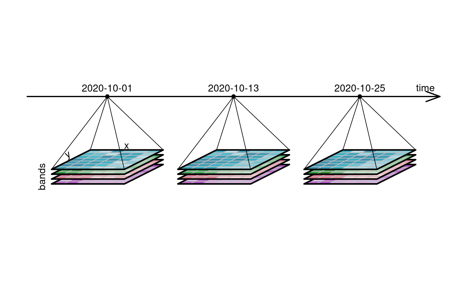
@fig-cube4d depicts a four-dimensional raster data
cube [@appel2019demand], where three-dimensional raster data cubes with a spectral
dimension ("bands") are organised along a fourth dimension, a time
axis. Colour image data always has three bands (blue, green, red),
and this example has a fourth band (near infrared, NIR), which is
commonly found in spectral remote sensing data.
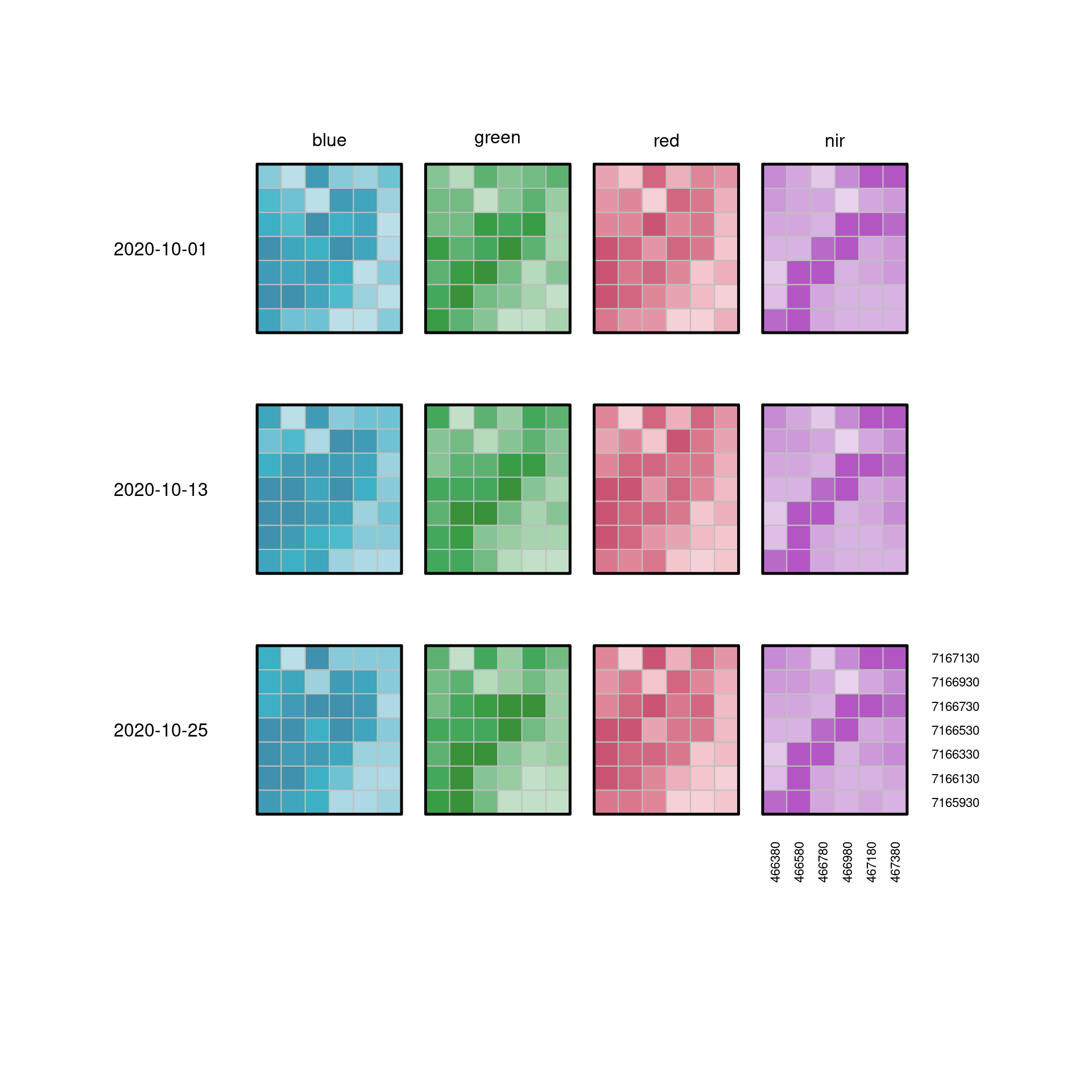
@fig-cube4d2 shows exactly the same data, but layed out
flat as a facet plot (or scatterplot matrix), where two dimensions
($x$ and $y$) are aligned with (or nested within) the dimensions
_bands_ and _time_, respectively.
```{r fig-cube4d2, echo=!knitr::is_latex_output()}
#| fig.cap: "Four-dimensional raster data cube layed out flat over two dimensions"
#| code-fold: true
#| fig.height: 10
#| fig.width: 10
# flat ----
xlabels <- seq(attr(warped, "dimensions")[[1]]$offset + attr(warped, "dimensions")[[1]]$delta / 2, length.out = attr(warped, "dimensions")[[1]]$to, by = attr(warped, "dimensions")[[1]]$delta)
ylabels <- seq(attr(warped, "dimensions")[[2]]$offset + attr(warped, "dimensions")[[2]]$delta / 2, length.out = attr(warped, "dimensions")[[2]]$to, by = attr(warped, "dimensions")[[2]]$delta)

print_labels <- function(x, y, off, lab, horizontal, cex = 1) {
  if(horizontal) { # x
    for(i in 0:(length(lab)-1)) {
      text(x + i*off, y, lab[i+1], cex = cex, srt = 90)
    }
  } else { # y
    lab <- lab[length(lab):0]
    for(i in 0:(length(lab)-1)) {
      text(x, y + i*off, lab[i+1], cex = cex)
    }
  }
}

# before: width=1000, xlim(-2, 33), date labels x=31
plot.new()
# par(mar = c(0,0,0,0))
par(mar = c(3,0,0,0))
plot.window(xlim = c(-2, 40), ylim = c(0, 25), asp = 1)
pl(f, 7, 0, pal = blues, m = b1)
pl(f, 7, 10, pal = blues, m = b2)
pl(f, 7, 20, pal = blues, m = b3)
pl(f, 14, 0, pal = greens, m = g1)
pl(f, 14, 10, pal = greens, m = g2)
pl(f, 14, 20, pal = greens, m = g3)
pl(f, 21, 0, pal = reds, m = r1)
pl(f, 21, 10, pal = reds, m = r2)
pl(f, 21, 20, pal = reds, m = r3)
pl(f, 28, 0, pal = purples, m = n1)
pl(f, 28, 10, pal = purples, m = n2)
pl(f, 28, 20, pal = purples, m = n3)
print_labels(28.5, -2, 1, xlabels, horizontal = TRUE, cex = 0.7)
print_labels(36, 0.5, 1, ylabels, horizontal = FALSE, cex = 0.7)
# arrows(6, 27, 6, 0, angle = 20, lwd = 2)
# text(5, 14, "time", srt = 90, col = "black")
text(10, 28, "blue", col = "black")
text(17, 28, "green", col = "black")
text(24, 28, "red", col = "black")
text(31, 28, "nir", col = "black")
text(3, 23.5, "2020-10-01", col = "black")
text(3, 13.5, "2020-10-13", col = "black")
text(3, 3.5, "2020-10-25", col = "black")
```
## Dimensions, attributes, and support
\index{data cube!dimensions}
\index{data cube!attributes}
\index{data cube!support}
Phenomena in space and time can be thought of as functions
with _domain_ space and time, and with _range_ one or more observed
attributes. For clearly identifiable discrete events or objects,
the range is typically discrete, and precise delineation involves
describing the precise coordinates where a thing starts or stops,
which is best suited by vector geometries. For continuous phenomena,
variables that take on a value everywhere such as air temperature
or land use type, there are infinitely many values to represent and
a common approach is to discretise space and time _regularly_ over
the spatiotemporal domain (extent) of interest. This leads to a
number of familiar data structures:
* time series, depicted as time lines for functions of time
* image or raster data for two-dimensional spatial data
* time sequences of images for dynamic spatial data
The third form of this, where a variable $Z$ depends on $x$, $y$
and $t$, as in
$$Z = f(x, y, t)$$
is the archetype of a spatiotemporal array or _data cube_: the shape
of the volume where points regularly discretising the domain forms a
cube. We call the variables that form the range (here: $x, y, t$) the
cube _dimensions_. Data cubes may have multiple attributes, as in
$$\{Z_1,Z_2,...,Z_p\} = f(x, y, t)$$
and if $Z$ is functional, for instance reflectance values measured over
the electromagnetic spectrum, the spectral wavelengths $\lambda$
may form an additional dimension, as in $Z = f(x,y,t,\lambda)$.
@sec-switching discusses the alternative of representing
colour bands as attributes.
Multiple time dimensions arise for instance when making forecasts for
different times in the future $t'$ at different times $t$, or when
time is split over multiple dimensions (as in year, day-of-year,
and hour-of-day). The most general definition of a data cube is a
functional mapping from $n$ dimensions to $p$ attributes:
$$\{Z_1,Z_2,...,Z_p\} = f(D_1,D_2,...,D_n)$$
Here, we will consider any dataset with one or more space dimensions
and zero or more time dimensions as data cubes. That includes:
* simple features (@sec-simplefeatures)
* time series for sets of features
* raster data
* multi-spectral raster data (images)
* time series of multi-spectral raster data (video)
\index{raster data cube}
\index{data cube!raster dimensions}
\index{data cube!vector geometry dimension}
\index{vector data cube}
### Regular dimensions, GDAL's geotransform
\index{data cube!regular dimensions}
\index{dimension!regular}
\index{GDAL!geotransform}
Data cubes are usually stored in multi-dimensional arrays, and the
usual relationship between 1-based array index $i$ and an associated
regularly discretised dimension variable $x$ is
$$x = o_x + (i-1) d_x$$
with $o_x$ the origin, and $d_x$ the grid spacing for this dimension.
For more general cases like those in Figures
[-@fig-rastertypes01] b-c, the relation between $x$ and $y$
and array indexes $i$ and $j$ is
$$x = o_x + (i-1) d_x + (j-1) a_1$$
$$y = o_y + (i-1) a_2 + (j-1) d_y$$
With two parameters $a_1$ and $a_2$ for rotation or affine transformation; this is the so-called
_geotransform_ as used in GDAL. When $a_1=a_2=0$, this
reduces to the regular raster of @fig-rastertypes01 a
with square cells if $d_x = d_y$.
For integer indexes, the coordinates are that of the starting _edge_
of a grid cell, and the cell area (pixel) spans a range corresponding to
index values ranging from $i$ (inclusive) to $i+1$ (exclusive).
For most common imagery formats, $d_y$ is negative,
indicating that image row index increases with decreasing $y$
values (southward). To get the $x$- and $y$-coordinate of the grid
cell _centre_ of the top left grid cell (in case of a negative $d_y$),
we use $i=1.5$ and $j=1.5$.
For rectilinear rasters, a table that maps array index to dimension
values is needed. NetCDF files for instance always store all values
of spatial dimension (coordinate) variables that may correspond to
the centre or offset of spatial grid cells, and in addition
may store grid cell boundaries (to define rectilinear dimensions
or to disambiguate the relation of the coordinate variable values
to the cell boundaries).
\index{raster!rectilinear}
\index{NetCDF}
For curvilinear rasters, an array that maps every combination of $i,j$
into $x,y$ pairs is needed, or a parametric function that does this
(a projection or its inverse). NetCDF files often provide both,
when available. GDAL calls such arrays _geolocation arrays_, and has
extensive support for transformations involving them.
\index{raster!curvilinear}
\index{GDAL!geolocation arrays}
### Support along cube dimensions
\index{data cube!dimension!support}
\index{support!data cube}
\index{support!dimension}
\index{support!temporal}
@sec-agr defined _spatial_ support of an attribute variable
as the size (length, area, volume) of a geometry associated with a particular
observation or prediction. The same notion
applies to temporal support. Although time is rarely reported by
explicit time periods having a start- and end-time, in many cases
either the time stamp implies a period (ISO-8601 uses
"2021" for the full year, "2021-01" for the full month) or the time
period is taken as the period from the time stamp of the current
record up to but not including the time stamp of the next record.
An example is MODIS satellite imagery, where vegetation indexes (NDVI
and EVI) are available as 16-day composites, meaning that over 16-day
periods all available imagery is aggregated into a single image; such
composites have temporal "block support". Sentinel-2 or Landsat-8
data on the other hand are "snapshot" images and have temporal
"point support". When temporally aggregating data with temporal
point support, for instance to monthly values, all images
falling in the target time interval are selected. When aggregating temporal block
support imagery such as the MODIS 16-day composite, one might
weigh images according to the amount of overlap of the 16-day
composite period and the target period, similar to area-weighted
interpolation [@sec-area-weighted] but over the time dimension.
## Operations on data cubes {#sec-dcoperations}
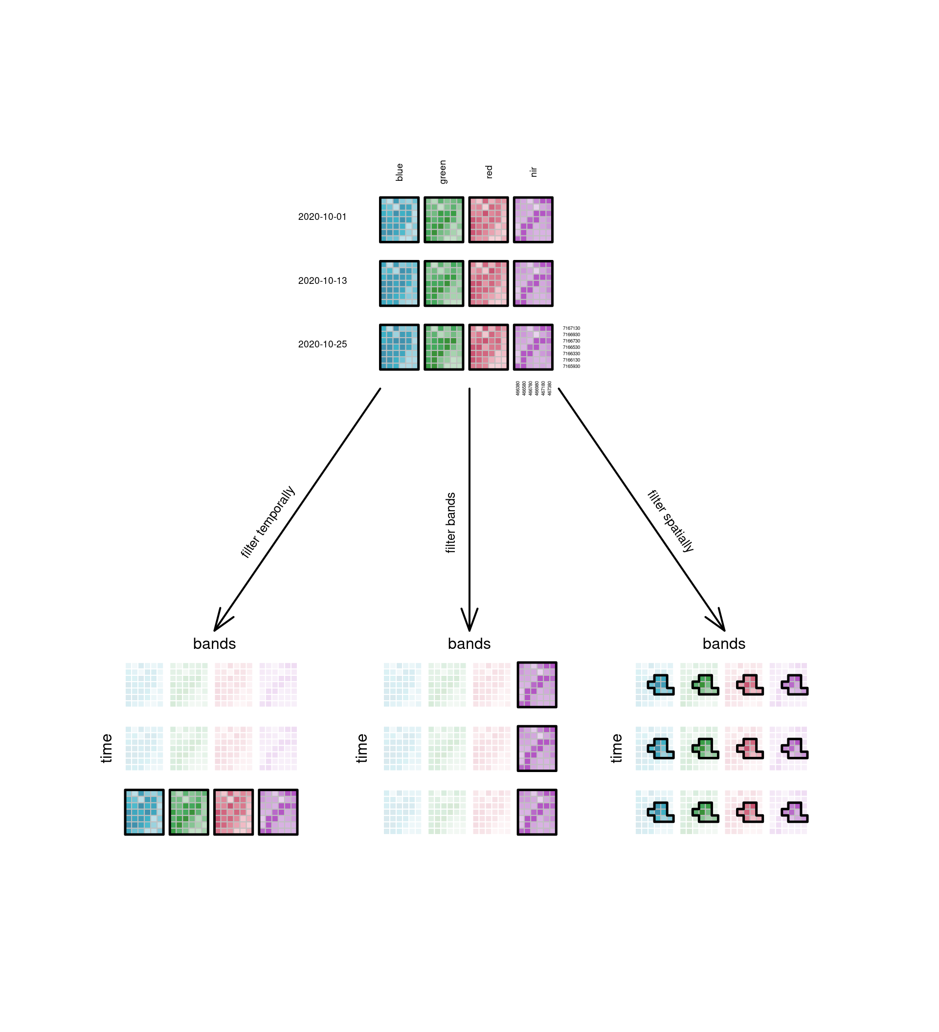
### Slicing a cube: filter
\index{data cube!filter}
Data cubes can be sliced into sub-cubes by fixing a dimension at
a particular value. @fig-cube4filter shows the sub-cubes obtained
by doing this with the temporal, spectral, or spatial dimension. In
this figure, the spatial filtering does not happen by fixing a
single spatial dimension at a particular value, but by selecting a
particular sub-region, which is a more common operation. Fixing $x$
or $y$ would give a sub-cube along a transect of constant $x$ or $y$,
which can be used to show a Hovmöller diagram, where an attribute is
plotted (coloured) in the space of one space and one time dimension.
```{r fig-cube4filter, echo=!knitr::is_latex_output()}
#| fig.width: 10
#| fig.height: 11
#| fig.cap: "Data cube filtering by time, band or spatially"
#| code-fold: true
# filter ----
# mask <- matrix(c(rep(NA, 26), 1,NA,1,NA,1,1,1, rep(NA, 9)), ncol = 7)
mask <- matrix(c(NA,NA,NA,NA,NA,NA,
                 NA,NA,NA,NA,NA,NA,
                 NA,NA,NA, 1, 1, 1,
                 NA,NA, 1, 1, 1,NA,
                 NA,NA,NA, 1, 1,NA,
                 NA,NA,NA,NA,NA,NA,
                 NA,NA,NA,NA,NA,NA), ncol = 7)

print_grid <- function(x, y) {
  pl(f, 0+x, 0+y, pal = blues, m = b1)
  pl(f, 0+x, 10+y, pal = blues, m = b2)
  pl(f, 0+x, 20+y, pal = blues, m = b3)
  pl(f, 7+x, 0+y, pal = greens, m = g1)
  pl(f, 7+x, 10+y, pal = greens, m = g2)
  pl(f, 7+x, 20+y, pal = greens, m = g3)
  pl(f, 14+x, 0+y, pal = reds, m = r1)
  pl(f, 14+x, 10+y, pal = reds, m = r2)
  pl(f, 14+x, 20+y, pal = reds, m = r3)
  pl(f, 21+x, 0+y, pal = purples, m = n1)
  pl(f, 21+x, 10+y, pal = purples, m = n2)
  pl(f, 21+x, 20+y, pal = purples, m = n3)
}
print_alpha_grid <- function(x,y, alp = 0.2, geom = FALSE) {
  pl(f, 0+x, 0+y, pal = alpha(blues, alp), print_geom = geom,  m = b1, border = 1)
  pl(f, 0+x, 10+y, pal = alpha(blues, alp), print_geom = geom,  m = b2, border = 1)
  pl(f, 0+x, 20+y, pal = alpha(blues, alp), print_geom = geom,  m = b3, border = 1)
  pl(f, 7+x, 0+y, pal = alpha(greens, alp), print_geom = geom,  m = g1, border = 1)
  pl(f, 7+x, 10+y, pal = alpha(greens, alp), print_geom = geom,  m = g2, border = 1)
  pl(f, 7+x, 20+y, pal = alpha(greens, alp), print_geom = geom,  m = g3, border = 1)
  pl(f, 14+x, 0+y, pal = alpha(reds, alp), print_geom = geom,  m = r1, border = 1)
  pl(f, 14+x, 10+y, pal = alpha(reds, alp), print_geom = geom,  m = r2, border = 1)
  pl(f, 14+x, 20+y, pal = alpha(reds, alp), print_geom = geom,  m = r3, border = 1)
  pl(f, 21+x, 0+y, pal = alpha(purples, alp), print_geom = geom,  m = n1, border = 1)
  pl(f, 21+x, 10+y, pal = alpha(purples, alp), print_geom = geom,  m = n2, border = 1)
  invisible(pl(f, 21+x, 20+y, pal = alpha(purples, alp), print_geom = geom,  m = n3, border = 1))
}

print_grid_filter <- function(x, y) {
  pl(f, 0+x, 0+y, pal = blues, m = matrix(b1[mask == TRUE], ncol = 7))
  pl(f, 0+x, 10+y, pal = blues, m = matrix(b2[mask == TRUE], ncol = 7))
  pl(f, 0+x, 20+y, pal = blues, m = matrix(b3[mask == TRUE], ncol = 7))
  pl(f, 7+x, 0+y, pal = greens, m = matrix(g1[mask == TRUE], ncol = 7))
  pl(f, 7+x, 10+y, pal = greens, m = matrix(g2[mask == TRUE], ncol = 7))
  pl(f, 7+x, 20+y, pal = greens, m = matrix(g3[mask == TRUE], ncol = 7))
  pl(f, 14+x, 0+y, pal = reds, m = matrix(r1[mask == TRUE], ncol = 7))
  pl(f, 14+x, 10+y, pal = reds, m = matrix(r2[mask == TRUE], ncol = 7))
  pl(f, 14+x, 20+y, pal = reds, m = matrix(r3[mask == TRUE], ncol = 7))
  pl(f, 21+x, 0+y, pal = purples, m = matrix(n1[mask == TRUE], ncol = 7))
  pl(f, 21+x, 10+y, pal = purples, m = matrix(n2[mask == TRUE], ncol = 7))
  pl(f, 21+x, 20+y, pal = purples, m = matrix(n3[mask == TRUE], ncol = 7))
}

print_grid_time_filter <- function(x, y) { # 3x1, 28x7
  pl(f, 0+x, 10+y, pal = blues, m = b3)
  pl(f, 7+x, 10+y, pal = greens, m = g3)
  pl(f, 14+x, 10+y, pal = reds, m = r3)
  pl(f, 21+x, 10+y, pal = purples, m = n3)
}

print_grid_bands_filter <- function(x, y, pal = greys) { # 1x3 6x27
  pl(f, 0+x, 0+y, pal = pal, m = n1)
  pl(f, 0+x, 10+y, pal = pal, m = n2)
  pl(f, 0+x, 20+y, pal = pal, m = n3)
}

# build exactly like reduce
plot.new()
par(mar = c(3,3,3,3))
x <- 120
y <- 100
down <- 0
plot.window(xlim = c(0, x), ylim = c(0, y), asp = 1)
print_grid(x/2-28/2,y-27)
print_alpha_grid((x/3-28)/2, 0-down) # alpha grid
print_grid_time_filter((x/3-28)/2, -10-down) # select 3rd
print_alpha_grid(x/3+((x/3-6)/2) -10.5, 0-down) # alpha grid
print_grid_bands_filter(x/3+((x/3-12.4)), 0-down, pal = purples)
print_alpha_grid(2*(x/3)+((x/3-28)/2), 0-down) # alpha grid
print_grid_filter(2*(x/3)+((x/3-28)/2), 0-down)
text(3, 13.5-down, "time", srt = 90, col = "black")
text(43, 13.5-down, "time", srt = 90, col = "black")
text(83, 13.5-down, "time", srt = 90, col = "black")
text(20, 30, "bands", col = "black")
text(60, 30, "bands", col = "black")
text(100, 30, "bands", col = "black")
arrows(x/2-28/2,y-30, x/6,32, angle = 20, lwd = 2)
arrows(x/2,y-30, x/2,32, angle = 20, lwd = 2)
arrows(x/2+28/2,y-30, 100, 32, angle = 20, lwd = 2)
# points(seq(1,120,10), seq(1,120,10))
text(28.5,49, "filter temporally", srt = 55.5, col = "black", cex = 0.8)
text(57,49, "filter bands", srt = 90, col = "black", cex = 0.8)
text(91.5,49, "filter spatially", srt = -55.5, col = "black", cex = 0.8)
print_labels(x = x/2-28/2 + 3, y = y+4, off = 7, lab = c("blue", "green", "red", "nir"),
             horizontal = TRUE, cex = 0.6)
print_labels(x = x/2-28/2 - 9, y = y-23, off = 10, lab = c("2020-10-01", "2020-10-13", "2020-10-25"),
             horizontal = FALSE, cex = 0.6)
print_labels(x = x/2-28/2 + 21.5, y = y-30, off = 1, lab = xlabels,
             horizontal = TRUE, cex = 0.3)
print_labels(x = x/2-28/2 + 30, y = y-26.5, off = 1, lab = ylabels,
             horizontal = FALSE, cex = 0.3)
```
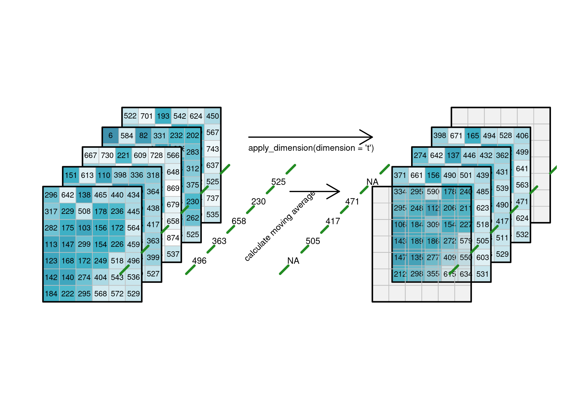
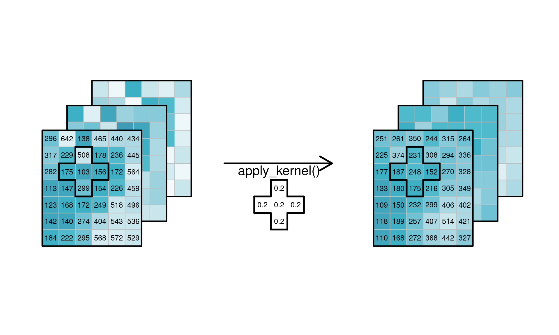
### Applying functions to dimensions {#sec-applydimension}
\index{data cube!apply function to dimension}
\index{dimension!apply function to dimension}
A common analysis involves applying a function over one or more
cube dimensions. Simple cases arise where a function such as `abs`,
`sin`, or `sqrt` is applied to all values in the cube, or when a function
takes all values in the cube and returns a single scalar, such as when
computing the mean or maximum value over the entire cube. Other
options include applying the function to selected dimensions,
such as applying a _temporal_ low-pass filter to every individual
(pixel/band) time series as shown in @fig-cube4apply1,
or applying a _spatial_ low-pass filter to every spatial
slice for every band/time combination, shown in
@fig-cube4apply2.
```{r fig-cube4apply1, echo=!knitr::is_latex_output()}
#| fig.width: 10
#| fig.height: 7
#| fig.cap: "Low-pass filtering of time series"
#| code-fold: true
print_text = function(s, x, y, m) {
  # m <- t(m) # transverse for correct order
  # print(m)
  r <- rep(seq(0.5, 5.5, 1), 7)
  r <- r + x # consider offsets
  u <- c(rep(0.5, 6), rep(1.5, 6), rep(2.5, 6),
         rep(3.5, 6), rep(4.5, 6), rep(5.5, 6), rep(6.5, 6))
  u <- u + y # offset
  tab <- matrix(c(r,u), nrow = 42, byrow = FALSE) # make point table
  for (i in 1:42) {
    #text(tab[i, 1], tab[i, 2], labels = paste0("", m[i]), cex = 1.1)
    text(tab[i, 1], tab[i, 2], labels = paste0("", m[i]), cex = 0.8)
    }
}
time_arrow_seg <- matrix(c(c(-1.0, 0.3, 1.5, 2.7, 3.9, 5.1), c(-1.0, 0.3, 1.5, 2.7, 3.9, 5.1),
                           c(-0.5, 0.7, 1.9, 3.1, 4.3, 5.6), c(-0.5, 0.7, 1.9, 3.1, 4.3, 5.6)), ncol = 4)
time_arrow_flag_seg <- matrix(c(c(-1.0, 1.5, 2.7, 3.9), c(-1.0, 1.5, 2.7, 3.9),
                                c(0.7, 1.9, 3.1, 5.6), c(0.7, 1.9, 3.1, 5.6)), ncol = 4)

b11 <- b2 - t1
b12 <- b1 - t2 + t1

brks <- seq(0, 1000, 50)
# png("exp_apply_ts.png", width = 2400, height = 1000, pointsize = 24)
plot.new()
par(mar = c(2,2,2,2))
x <- 30
y <- 10 # 7.5
plot.window(xlim = c(0, x), ylim = c(0, y), asp = 1)
pl(f, 4.8, 3.8, pal = blues, m = b3, breaks = brks)
print_text(s, 4.8, 3.8, m = b3)
pl(f, 3.6, 2.6, pal = blues, m = b11, breaks = brks)
print_text(s, 3.6, 2.6, m = b11)
pl(f, 2.4, 1.4, pal = blues, m = b12, breaks = brks)
print_text(s, 2.4, 1.4, m = b12)
pl(f, 1.2, .2, pal = blues, m = b2, breaks = brks)
print_text(s, 1.2, .2, m = b2)
pl(f, 0, -1, pal = blues, m = b1, breaks = brks)
print_text(s, 0, -1, m = b1) # print text on left first stack
pl(f, 24.8, 3.8, pal = alpha(greys, 0.1), m = matrix(rep("NA", 42), ncol = 7))
pl(f, 23.6, 2.6, pal = blues, m = (b12 + b11 + b3) / 3, breaks = brks)
print_text(s, 23.6, 2.6, m = floor((b12 + b11 + b3) / 3))
pl(f, 22.4, 1.4, pal = blues, m = (b2 + b12 + b11) / 3, breaks = brks)
print_text(s, 22.4, 1.4, m = floor((b2 + b12 + b11) / 3))
pl(f, 21.2, .2, pal = blues, m = (b1 + b2 + b12) / 3, breaks = brks)
print_text(s, 21.2, .2, m = floor((b1 + b2 + b12) / 3))
pl(f, 20, -1, pal = alpha(greys, 0.1), m = matrix(rep("NA", 42), ncol = 7))
print_segments(5.7, 1.7, seg = time_arrow_seg, col = "forestgreen")
arrows(12.5, 9, 20, 9, lwd = 2)
cex <- .9
text(16.3, 8.3, "apply_dimension(dimension = 't')", cex = cex)
print_segments(9.7, 1.7, time_arrow_seg, col = "forestgreen") # draw ma explanation
text(-0.5 + 10, -0.5 + 2, "496", cex = cex)
text(.7 + 10, .7 + 2, "363", cex = cex)
text(1.9 + 10, 1.9 + 2, "658", cex = cex)
text(3.1 + 10, 3.1 + 2, "230", cex = cex)
text(4.3 + 10, 4.3 + 2, "525", cex = cex)
t_formula <- expression("t"[n]*" = (t"[n-1]*" + t"[n]*" + t"[n+1]*") / 3")
# text(13.8, 3, t_formula, srt = 45, cex = 1.2)
text(14.4, 3.6, "calculate moving average", srt = 45, cex = cex)
arrows(15, 5.7, 18, 5.7, lwd = 2)
print_segments(15.4, 1.7, seg = time_arrow_seg, col = "forestgreen") # draw ma explanation
text(-0.5 + 15.7, -0.5 + 2, "NA", cex = cex)
text(.7 + 15.7, .7 + 2, "505", cex = cex)
text(1.9 + 15.7, 1.9 + 2, "417", cex = cex)
text(3.1 + 15.7, 3.1 + 2, "471", cex = cex)
text(4.3 + 15.7, 4.3 + 2, "NA", cex = cex)
print_segments(25.7, 1.7, seg = time_arrow_seg, col = "forestgreen")
```
```{r fig-cube4apply2, echo=!knitr::is_latex_output()}
#| fig.height: 6
#| fig.width: 10
#| fig.cap: "Low pass filtering of spatial slices"
#| code-fold: true
# apply ----

abs_brks <- seq(-500,500, 50)
abs_pal <- sequential_hcl(n = 20, h1 = 211, c1 = 80, l1 = 30, l2 = 100, p1 = 1.2)

vNeumann_seg <- matrix(c(c(0,0,1,1,2,2,1,1,0,0,-1,-1), c(0,-1,-1,0,0,1,1,2,2,1,1,0),
                         c(0,1,1,2,2,1,1,0,0,-1,-1,0), c(-1,-1,0,0,1,1,2,2,1,1,0,0)), ncol = 4)

apply_filter <- function(input, pad = TRUE, padValue = 1) {
  ras <- raster::focal(raster::raster(input), w = matrix(c(0,0.2,0, 0.2,0.2,0.2, 0,0.2,0), ncol = 3), pad = pad, padValue = padValue)
  ras <- raster::as.matrix(ras)
  ras[ras == "NaN"] <- -999
  return(floor(ras))
}

brks <- seq(0, 1000, 50)
plot.new()
par(mar = c(0,2,0,0))
x = 30
y = 7.5
plot.window(xlim = c(0, x), ylim = c(0, y), asp = 1)
pl(f, 3, 2, pal = blues, m = b3, breaks = brks)
pl(f, 1.5, .5, pal = blues, m = b2, breaks = brks)
pl(f, 0, -1, pal = blues, m = b1, breaks = brks)
print_text(s, 0, -1, m = b1) # print text on left first stack
print_segments(2, 3, seg = vNeumann_seg, lwd = 3)
pl(f, 23, 2, pal = blues, m = apply_filter(b3), breaks = brks)
pl(f, 21.5, 0.5, pal = blues, m = apply_filter(b2), breaks = brks)
pl(f, 20, -1, pal = blues, m = apply_filter(b1), breaks = brks)
print_text(s, 20, -1, m = apply_filter(b1)) # set pad = FALSE for -99
print_segments(22, 3, seg = vNeumann_seg, lwd = 3)
arrows(11, 4, 17.5, 4, lwd = 3)
text(14.3, 3.5, "apply_kernel()", cex = 1.4)
print_segments(13.8, 1, seg = vNeumann_seg, lwd = 3)
cex = .8
text(14.3, 1.5, "0.2", cex = cex)
text(13.3, 1.5, "0.2", cex = cex)
text(15.3, 1.5, "0.2", cex = cex)
text(14.3, 2.5, "0.2", cex = cex)
text(14.3, .5, "0.2", cex = cex)
```
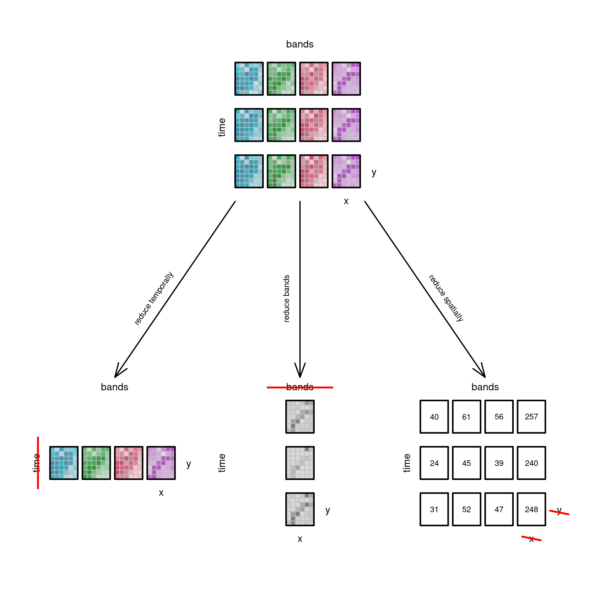
### Reducing dimensions {#sec-reducedimension}
\index{dimension!reduce}
\index{reduce dimension}
\index{data cube!reduce dimension}
When applying function `mean` to an entire data cube, all dimensions
vanish: the resulting "data cube" has dimensionality zero. We
can also apply functions to a limited set of dimensions such that
selected dimensions vanish, or are _reduced_. We already saw that
filtering is a special case of this, but more in general we could
for instance compute the maximum of every time series, the mean over
every spatial slice, or a band index such as NDVI that summarises
different spectral values into a single new "band" with the index
value. @fig-cube4reduce illustrates these options.
```{r fig-cube4reduce, echo=!knitr::is_latex_output()}
#| fig.width: 10
#| fig.height: 10
#| fig.cap: "Reducing data cube dimensions"
#| code-fold: true
# reduce ----

# calc mean over time
timeB <- (b1 + b2 + b3) / 3
timeG <- (g1 + g2 + g3) / 3
timeR <- (r1 + r2 + r3) / 3
timeN <- (n1 + n2 + n3) / 3

print_grid_time <- function(x, y) { # 3x1, 28x7
  pl(f, 0+x, 10+y, pal = blues, m = timeB)
  pl(f, 7+x, 10+y, pal = greens, m = timeG)
  pl(f, 14+x, 10+y, pal = reds, m = timeR)
  pl(f, 21+x, 10+y, pal = purples, m = timeN)
}

# calc ndvi
ndvi1 <- (n1 - r1) / (n1 + r1)
ndvi2 <- (n2 - r2) / (n2 + r2)
ndvi3 <- (n3 - r3) / (n3 + r3)

print_grid_bands <- function(x, y, pal = greys) { # 1x3 6x27
  pl(f, 0+x, 0+y, pal = pal, m = ndvi1)
  pl(f, 0+x, 10+y, pal = pal, m = ndvi2)
  pl(f, 0+x, 20+y, pal = pal, m = ndvi3)
}

plte = function(s, x, y, add = TRUE, randomize = FALSE, pal, m) {
  attr(s, "dimensions")[[1]]$offset = x
  attr(s, "dimensions")[[2]]$offset = y
  # m = r[[1]][y + 1:nrow,x + 1:ncol,1]
  # dim(m) = c(x = nrow, y = ncol) # named dim
  # s[[1]] = m
  # me <- floor(mean(s[[1]]))
  me <- floor(mean(m))
  if (me[1] > 100) { # in case non-artificial grids with very high
    me <- m / 10     # numbers are used, make them smaller
    me <- floor(mean(me))
  }
  text(x,y,me,cex = 0.8)
}

print_grid_spat <- function(x, y) {
  x = x + 3
  y = y + 3.5
  plte(s, 0+x, 0+y, pal = blues, m = b1)
  plte(s, 0+x, 10+y, pal = blues, m = b2)
  plte(s, 0+x, 20+y, pal = blues, m = b3)
  plte(s, 7+x, 0+y, pal = greens, m = g1)
  plte(s, 7+x, 10+y, pal = greens, m = g2)
  plte(s, 7+x, 20+y, pal = greens, m = g3)
  plte(s, 14+x, 0+y, pal = reds, m = r1)
  plte(s, 14+x, 10+y, pal = reds, m = r2)
  plte(s, 14+x, 20+y, pal = reds, m = r3)
  plte(s, 21+x, 0+y, pal = purples, m = n1)
  plte(s, 21+x, 10+y, pal = purples, m = n2)
  plte(s, 21+x, 20+y, pal = purples, m = n3)
}

# png("exp_reduce.png", width = 1200, height = 1000, pointsize = 32)
plot.new()
#par(mar = c(3,3,3,3))
par(mar = c(3,0,2,0))
x = 120
y = 100
plot.window(xlim = c(0, x), ylim = c(0, y), asp = 1)
print_grid(x/2-28/2,y-27)
# print_alpha_grid((x/3-28)/2, 0) # alpha grid
print_grid_time((x/3-28)/2, 0) # off = 5.5
# print_alpha_grid(x/3+((x/3-6)/2) -10.5, 0) # alpha grid
print_grid_bands(x/3+((x/3-6)/2), 0)
print_alpha_grid(2*(x/3)+((x/3-28)/2), 0, alp = 0, geom = TRUE) # alpha grid
print_grid_spat(2*(x/3)+((x/3-28)/2), 0)
text(3, 13.5, "time", srt = 90, col = "black")
#segments(3.6, 8, 3.7, 19, col = "red", lwd=3)
segments(3.4, 8, 3.4, 19, col = "red", lwd = 3)
text(43, 13.5, "time", srt = 90, col = "black")
text(83, 13.5, "time", srt = 90, col = "black")
text(20, 30, "bands", col = "black")
text(60, 30, "bands", col = "black")
segments(53,29.8, 67,29.8, col = "red", lwd = 3)
text(100, 30, "bands", col = "black")
text(30, 7, "x", col = "black")
text(36, 13, "y", col = "black")
text(60, -3, "x", col = "black")
text(66, 3, "y", col = "black")
text(110, -3, "x", col = "black")
text(116, 3, "y", col = "black")
segments(108,-2.4, 112,-3.2, col = "red", lwd = 3)
segments(114,3.2, 118,2.4, col = "red", lwd = 3)
text(60, y+4, "bands", col = "black") # dim names on main
text(43, y-14, "time", srt = 90, col = "black")
text(x/2-28/2 + 24, y-30, "x", col = "black")
text(x/2-28/2 + 30, y-24, "y", col = "black")
arrows(x/2-28/2,y-30, x/6,32, angle = 20, lwd = 2)
arrows(x/2,y-30, x/2,32, angle = 20, lwd = 2)
arrows(x/2+28/2,y-30, 100, 32, angle = 20, lwd = 2)
# points(seq(1,120,10), seq(1,120,10))
text(28.5,49, "reduce temporally", srt = 55.5, col = "black", cex = 0.8)
text(57,49, "reduce bands", srt = 90, col = "black", cex = 0.8)
text(91.5,49, "reduce spatially", srt = -55.5, col = "black", cex = 0.8)
```
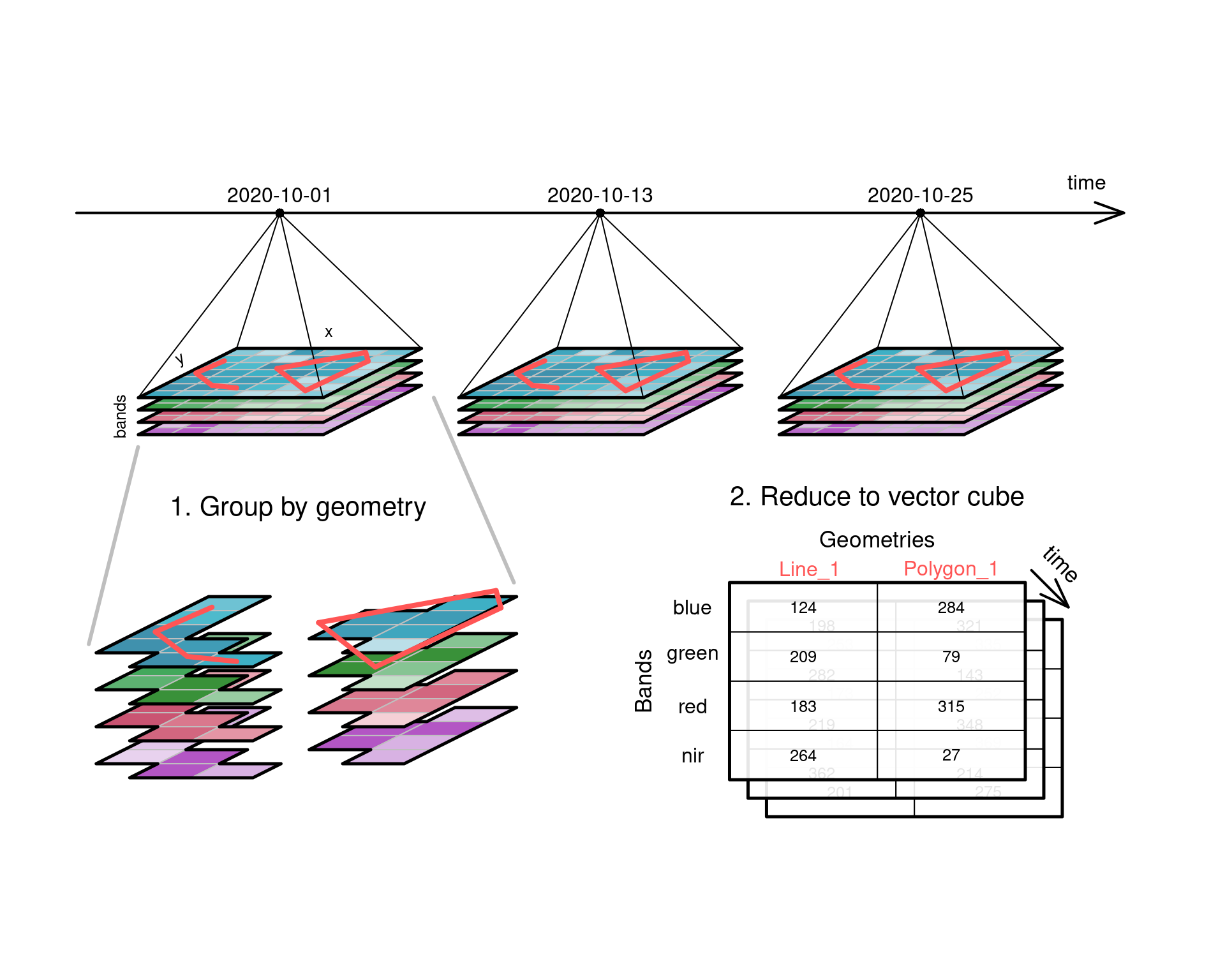
## Aggregating raster to vector cubes {#sec-vectordatacubes}
\index{data cube!aggregate to vector cube}
\index{aggregate!data cube}
@fig-cube4agg illustrates how a four-dimensional raster
data cube can be aggregated to a three-dimensional _vector data
cube_. Pixels in the raster are grouped by spatial intersection
with a set of vector geometries, and each group is then reduced
to a single value by an aggregation function such as `mean` or
`max`. In the example, the _two_ spatial dimensions $x$ and $y$
reduce to a single dimension, the one-dimensional sequence of feature
geometries, with geometries that are defined in the space of $x$
and $y$. Grouping geometries can also be `POINT` geometries, in
which case the aggregation function is obsolete as single values
at the `POINT` locations are _extracted_ by querying a pixel
value or by interpolating from the nearest pixels.
```{r fig-cube4agg, echo=!knitr::is_latex_output()}
#| fig.cap: "Aggregating a raster data cube to a vector data cube"
#| fig.width: 10
#| fig.height: 8
#| code-fold: true
# aggregate ----

mask_agg <- matrix(c(NA,NA,NA,NA,NA,NA,
                 NA, 1, 1,NA,NA,NA,
                  1, 1,NA,NA, 1,NA,
                  1,NA,NA, 1, 1,NA,
                  1,NA,NA, 1, 1,NA,
                  1,NA,NA,NA, 1,NA,
                 NA,NA,NA,NA,NA,NA), ncol = 7)

pl_stack_agg <- function(s, x, y, add = TRUE, nrM, imgY = 7, inner = 1) {
  # pl_stack that masks the added matrices
  # nrM is the timestep {1, 2, 3}, cause this function
  # prints all 4 bands at once
  attr(s, "dimensions")[[1]]$offset = x
  attr(s, "dimensions")[[2]]$offset = y
  # m = r[[1]][y + 1:nrow,x + 1:ncol,1]
  m <- eval(parse(text=paste0("n", nrM)))
  m <- matrix(m[mask_agg == TRUE], ncol = 7)
  s[[1]] = m[,c(imgY:1)] # turn around to have same orientation as flat plot
  plt(s, 0, TRUE,  pal = purples)
  m <- eval(parse(text=paste0("r", nrM)))
  m <- matrix(m[mask_agg == TRUE], ncol = 7)
  s[[1]] = m[,c(imgY:1)]
  plt(s, 1*inner, TRUE,  pal = reds)
  m <- eval(parse(text=paste0("g", nrM)))
  m <- matrix(m[mask_agg == TRUE], ncol = 7)
  s[[1]] = m[,c(imgY:1)]
  plt(s, 2*inner, TRUE,  pal = greens)
  m <- eval(parse(text=paste0("b", nrM)))
  m <- matrix(m[mask_agg == TRUE], ncol = 7)
  s[[1]] = m[,c(imgY:1)]
  plt(s, 3*inner, TRUE, pal = blues) # li FALSE
}

polygon_1 <- matrix(c(c(0.0, 5.1, 4.9,-2.3), c(0.0, 2.4, 3.1, 1.8),
                      c(5.1, 4.9,-2.3, 0.0), c(2.4, 3.1, 1.8, 0.0)), ncol = 4)

a <- make_dummy_stars(6, 7, 5, -1.14, -2.28)

print_vector_content <- function(x, y, cex = 0.8) {
  vec <- floor(rnorm(8, 250, 100))
  text( 0 + x,12 + y, vec[1], cex = cex)
  text( 0 + x, 8 + y, vec[2], cex = cex)
  text( 0 + x, 4 + y, vec[3], cex = cex)
  text( 0 + x, 0 + y, vec[4], cex = cex)
  text( 12 + x,12 + y, vec[5], cex = cex)
  text( 12 + x, 8 + y, vec[6], cex = cex)
  text( 12 + x, 4 + y, vec[7], cex = cex)
  text( 12 + x, 0 + y, vec[8], cex = cex)
}

print_ts <- function(off2, yoff2) {
  pl_stack(s, 0 + off2, yoff2, nrM = 3) # input 2
  pl_stack(s, off + off2, yoff2, nrM = 2)
  pl_stack(s, 2 * off + off2, yoff2, nrM = 1)
  arrows(-13 + off2, 14 + yoff2, 72 + off2, 14 + yoff2, angle = 20, lwd = 2)  # timeline
  heads <- matrix(c(3.5+off2, 3.5 + off + off2, 3.5 + 2*off + off2, 14+yoff2,14+yoff2,14+yoff2), ncol = 2)
  points(heads, pch = 16) # 4 or 16
  segments(c(-8, 7, 0, 15)+off2, c(-1,-1,3,3)+yoff2, 3.5+off2, 14+yoff2) # first stack pyramid
  segments(c(-8, 7, 0, 15) + off + off2, c(-1,-1,3,3)+yoff2, 3.5 + off + off2, 14+yoff2) # second stack pyramid
  segments(c(-8, 7, 0, 15) + 2*off + off2, c(-1,-1,3,3)+yoff2, 3.5 + 2*off + off2, 14+yoff2) # third stack pyramid
  text(7.5+off2, 4.3+yoff2, "x", col = "black", cex = secText)
  text(-9.5+off2, -2.5+yoff2, "bands", srt = 90, col = "black", cex = secText)
  text(-4.5+off2, 2+yoff2, "y", srt = 27.5, col = "black", cex = secText)
  text(69+off2, 15.5+yoff2+1, "time", col = "black")
  text(3.5+off2, 15.5+yoff2, "2020-10-01", col = "black")
  text(3.5 + off + off2, 15.5+yoff2, "2020-10-13", col = "black")
  text(3.5 + 2*off + off2, 15.5+yoff2, "2020-10-25", col = "black")
}

secText <- 0.8 # secondary text size (dimension naming)
off <- 26 # image stacks are always 26 apart
x <- 72 # png X
y <- 48 # png Y
yoff <- 30
plot.new()
par(mar = c(5,3,3,3))
plot.window(xlim = c(-5, x+4), ylim = c(-1, y), asp = 1)
print_ts(5, yoff)
col <- '#ff5555'
print_segments(10.57, yoff-.43, seg = polygon_1, col = col)
x = 3
segments(c(2, 0, -1.3)+x, c(-.2, 0, 1)+yoff, c(0, -1.3, 1)+x, c(0, 1, 2)+yoff, lwd = 4, col = col)
print_segments(10.57+off, yoff-.43, seg = polygon_1, col = col)
x = 3 + off
segments(c(2, 0, -1.3)+x, c(-.2, 0, 1)+yoff, c(0, -1.3, 1)+x, c(0, 1, 2)+yoff, lwd = 4, col = col)
print_segments(10.57+2*off, yoff-.43, seg = polygon_1, col = col)
x = 3 + 2 * off
segments(c(2, 0, -1.3)+x, c(-.2, 0, 1)+yoff, c(0, -1.3, 1)+x, c(0, 1, 2)+yoff, lwd = 4, col = col)
# old 75 28 poly 86.25, 27.15
pl_stack_agg(a, 5, 5, nrM = 1, inner = 3) # print masked enlargement
print_segments(16.25, 7.15, seg = polygon_1, by = 2, col = col)
x <- 1
y <- 8
segments(c(4, 0, -2.6)+x, c(-.4, 0, 2)+y, c(0, -2.6, 2)+x, c(0, 2, 4)+y, lwd = 4, col = col) # line in large
segments(-3, 25, -7, 9, lwd = 3, col = 'grey')
segments(21, 29, 27.5, 14, lwd = 3, col = 'grey')
text(10, 20, "1. Group by geometry", cex = 1.3)
vecM <- matrix(rep(1,8), ncol = 2)
text(57, 21, "2. Reduce to vector cube", cex = 1.3)
b <- make_dummy_stars(2, 4, 12, 4, 0)
pl(b, 48, -5, m = vecM, pal = alpha("white", 0.9), border = 0)
print_vector_content(54, -3)
pl(b, 46.5, -3.5, m = vecM, pal = alpha("white", 0.9), border = 0)
print_vector_content(52.5, -1.5)
pl(b, 45, -2, m = vecM, pal = alpha("white", 0.9), border = 0)
print_vector_content(51, 0)
text(51.5, 15, "Line_1", col = col)
text(63, 15, "Polygon_1", col = col)
text(57, 17.5, "Geometries", cex = 1.1)
text(42, 12, "blue")
text(42,  8, "green")
text(42,  4, "red")
text(42,  0, "nir")
text(38, 6, "Bands", srt = 90, cex = 1.1)
# arrows(13.5, -2, 13.5, -6, angle = 20, lwd = 3)
text(72, 15.5, "time", srt = 315, cex = 1.1)
arrows(69.5, 15, 72.5, 12, angle = 20, lwd = 2)
# print_segments(30, 35, seg = arrow_seg)
```
Further examples of vector data cubes include air quality data,
where we could have $PM_{10}$ measurements over two dimensions,
as a sequence of
* monitoring stations, and
* time intervals
or where we consider time series of demographic or epidemiological
data, consisting of (population, disease) counts, with number
of persons by
* region, for a sequence of $n$ regions
* age class, for $m$ age classes, and
* year, for $p$ years
which forms an array with $n m p$ elements.
For spatial data science, handling vector and raster data cubes
is extremely useful, because many variables are both spatially
and temporaly varying, and because we often want to either change
dimensions or aggregate them out, but in a fully flexible manner
and order. Examples of changing dimensions are:
* interpolating air quality measurements to values on a regular grid (raster; @sec-interpolation)
* estimating density maps from points or lines, for instance estimating the number of flights passing by per week within a range of 1 km (@sec-pointpatterns)
* aggregating climate model predictions to summary indicators for administrative regions
* combining Earth observation data from different sensors, such as MODIS (250~m pixels, every 16 days) with Sentinel-2 (10~m pixels, every 5 days)
Examples of aggregating one or more full dimensions are assessments of:
* which air quality monitoring stations indicate unhealthy conditions (time)
* which region has the highest increase in disease incidence (space, time)
* global warming (global change in degrees Celsius per decade)
## Switching dimension with attributes {#sec-switching}
\index{data cube!switch dimension attribute}
\index{dimension!switch with attribute}
When we accept that a dimension can also reflect an unordered,
categorical variable, then one can easily swap a set of attributes
for a single dimension, by replacing
$$\{Z_1,Z_2,...,Z_p\} = f(D_1,D_2,...,D_n)$$
with
$$Z = f(D_1,D_2,...,D_n, D_{n+1})$$
where $D_{n+1}$ has cardinality $p$ and has as labels (the names
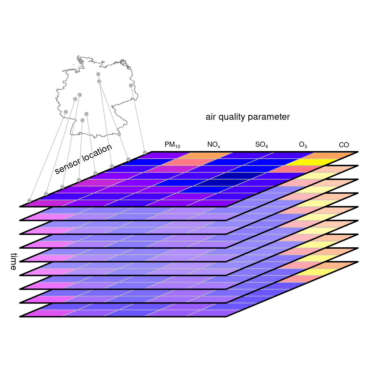
of) $Z_1,Z_2,...,Z_p$. @fig-aqdc shows a vector data
cube for air quality stations where one cube dimension reflects
air quality parameters. When the $Z_i$ have incompatible measurement
units, as in @fig-aqdc, one would have to take care
when reducing the "parameter" dimension $D_{n+1}$: numeric functions
like `mean` or `max` would be meaningless. Counting the number of
variables that exceed their respective threshold values may however
be meaningful.
```{r fig-aqdc, echo=!knitr::is_latex_output()}
#| fig.cap: "Vector data cube with air quality time series"
#| fig.height: 7
#| code-fold: true
set.seed(1331)
library(stars)
library(colorspace)
tif <- system.file("tif/L7_ETMs.tif", package = "stars")
r <- read_stars(tif)

nrow <- 5
ncol <- 8
#m = matrix(runif(nrow * ncol), nrow = nrow, ncol = ncol)
m <- r[[1]][1:nrow,1:ncol,1]
dim(m) <- c(x = nrow, y = ncol) # named dim
s <- st_as_stars(m)
# s
attr(s, "dimensions")[[1]]$delta = 3
attr(s, "dimensions")[[2]]$delta = -.5
attr(attr(s, "dimensions"), "raster")$affine = c(-1.2, 0.0)

plt <- function(x, yoffset = 0, add, li = TRUE) {
    attr(x, "dimensions")[[2]]$offset = attr(x, "dimensions")[[2]]$offset + yoffset
    l = st_as_sf(x, as_points = FALSE)
    pal = sf.colors(10)
    if (li)
        pal = lighten(pal, 0.3 + rnorm(1, 0, 0.1))
    if (! add)
        plot(l, axes = FALSE, breaks = "equal", pal = pal, reset = FALSE, border = grey(.75), key.pos = NULL, main = NULL, xlab = "time")
    else
        plot(l, axes = TRUE, breaks = "equal", pal = pal, add = TRUE, border = grey(.75))
    u = st_union(l)
    plot(st_geometry(u), add = TRUE, col = NA, border = 'black', lwd = 2.5)
}

pl <- function(s, x, y, add = TRUE, randomize = FALSE) {
  attr(s, "dimensions")[[1]]$offset = x
  attr(s, "dimensions")[[2]]$offset = y
  m = r[[1]][y + 1:nrow,x + 1:ncol,1]
  if (randomize)
    m = m[sample(y + 1:nrow),x + 1:ncol]
  dim(m) = c(x = nrow, y = ncol) # named dim
  s[[1]] = m
  plt(s, 0, add)
  plt(s, 1, TRUE)
  plt(s, 2, TRUE)
  plt(s, 3, TRUE)
  plt(s, 4, TRUE)
  plt(s, 5, TRUE)
  plt(s, 6, TRUE)
  plt(s, 7, TRUE)
  plt(s, 8, TRUE, FALSE)
}

# point vector data cube:
plot.new()
par(mar = c(5, 0, 5, 0))
plot.window(xlim = c(-10, 16), ylim = c(-2,12), asp = 1)
library(spacetime)
data(air)
de = st_geometry(st_normalize(st_as_sf(DE)))
#
pl(s, 0, 0, TRUE, randomize = TRUE)
de = de * 6 + c(-7, 9)
plot(de, add = TRUE, border = grey(.5))
text(-10, 0, "time", srt = -90, col = 'black')
text(-5,  7.5, "sensor location", srt = 25, col = 'black')
text( 7,  10.5, "air quality parameter", srt = 0, col = 'black')
text( 1.5,  8.5, expression(PM[10]), col = 'black', cex = .75)
text( 4.5,  8.5, expression(NO[x]), col = 'black', cex = .75)
text( 8,  8.5, expression(SO[4]), col = 'black', cex = .75)
text( 11,  8.5, expression(O[3]), col = 'black', cex = .75)
text( 14,  8.5, expression(CO), col = 'black', cex = .75)
# location points:
p <- st_coordinates(s[,1])
p[,1] <- p[,1]-1.4
p[,2] <- p[,2] + 8.2
points(p, col = grey(.7), pch = 16)
# centroids:
set.seed(131)
cent <- st_coordinates(st_sample(de, 8))
points(cent, col = grey(.7), pch = 16)
cent <- cent[rev(order(cent[,1])),]
seg <- cbind(p, cent[1:8,])
segments(seg[,1], seg[,2], seg[,3], seg[,4], col = 'grey')
```
Being able to swap dimensions to attributes flexibly and vice versa
leads to highly flexible analysis possibilities [@brown2010overview].
## Other dynamic spatial data {#sec-otherdynamic}
\index{trajectories}
\index{dynamic spatial data}
We have seen several dynamic raster and vector data examples
that match the data cube structure well. Other data examples
do less so: in particular spatiotemporal point patterns
(@sec-pointpatterns) and trajectories [movement data; for a recent
review, see @https://doi.org/10.1111/1365-2656.13116] are often more
straightforward to not handle as a data cube. Spatiotemporal point
patterns are the sets of spatiotemporal coordinates of events or
objects: accidents, disease cases, traffic jams, lightning strikes,
and so on. Trajectory data are time sequences of spatial locations of
moving objects (persons, cars, satellites, animals). For such data,
the primary information is in the coordinates, and shifting these
to a limited set of regularly discretised grid cells covering the
space may help some analysis, for instance to quickly explore patterns in
areas of higher densities, but the loss of the exact coordinates
also hinders a number of analysis approaches involving distance,
direction, or speed calculations. Nevertheless, for such data often
the first computational steps involves generation of data cube
representations by aggregating to a time-fixed spatial and/or
space-fixed temporal discretisation.
Using sparse array representations of data cubes to represent
point pattern or trajectory data, which is possible for instance with SciDB
[@brown2010overview] or TileDB [@tiledb], may strongly limit the
loss of coordinate accuracy by choosing dimensions that represent
an extremely dense grid, and storing only those grid cells that
contain data points. For trajectory data, such representations
would need to add a grouping dimension to identify individuals,
or individual sequences of consecutive movement observations.
## Exercises
Use words to solve the following exercises. If needed or relevant
use R code to illustrate the argument(s).
1. Why is it difficult to represent trajectories, sequences of
$(x,y,t)$ obtained by tracking moving objects, by data cubes as
described in this chapter?
2. In a socio-economic vector data cube with variables population,
life expectancy, and gross domestic product ordered by dimensions country and
year, which variables have block support for the spatial dimension,
and which have block support for the temporal dimension?
3. The Sentinel-2 satellites collect images in 12 spectral bands;
list advantages and disadvantages to represent them as (i) different
data cubes, (ii) a data cube with 12 attributes, one for each band,
and (iii) a single attribute data cube with a spectral dimension.
4. Explain why a curvilinear raster as shown in
@fig-rastertypes01 can be considered a special case of a
data cube.
5. Explain how the following problems can be solved with data cube
operations `filter`, `apply`, `reduce` and/or `aggregate`, and
in which order. Also mention for each which function is applied,
and what the dimensionality of the resulting data cube is (if any):
* from hourly $PM_{10}$ measurements for a set of air quality
monitoring stations, compute per station the amount of days
per year that the average daily $PM_{10}$ value exceeds
50 $\mu g/m^3$
* for a sequence of aerial images of an oil spill, find the
time at which the oil spill had its largest extent, and the
corresponding extent
* from a 10-year period with global daily sea surface temperature
(SST) raster maps, find the area with the 10% largest and 10%
smallest temporal trends in SST values.