# Introduction to spatial data
### Learning goals
- learn the different data types considered in spatial statistics, and get familiar with simple features, as well as with the difference between discrete and continuous variability in *space* and in *attributes*
- learn what spatial dependence is about, and cases where it can be ignored
- introduce spatial point patterns and processes
### Reading materials
From [Spatial Data Science: with applications in R](https://r-spatial.org/book/):
- Preface
- Chapter 1: Getting started
- Chapter 2: Coordinates
- Chapter 10: Statistical modelling of spatial data
### Exercises that can be prepared for the first day:
- Section 10.6: Exercises
::: {.callout-tip title="Summary"}
- Introduction to spatial data, support, coordinate reference systems
- Introduction to spatial statistical data types: point patterns, geostatistical data, lattice data; imagery, tracks/trajectories
- Is spatial dependence a fact? And is it a curse, or a blessing?
- Spatial sampling, design-based and model-based inference
- Intro to point patterns and point processes, observation window, first and second order properties
- Checklist for your spatial data
:::
## What is special about spatial data?
- **Location**. Does location always involve coordinates? Relative/absolute, qualitative/quantitative
- **Coordinates**. What are coordinates? Dimension(s), unit
- **Time**. If not explicit, there is an implicit time reference. Dimension(s), unit, datetime
- **Attributes**. *at* specific locations we measure (observe) specific properties
- Quite often, we want to know *where* things change (**space-time interactions**).
- **Reference systems** for space, time, and attributes: what are they?
- **Support**: if we have an attribute value associated with a line, polygon or grid cell:
- does the value summarise all values at points? (line/area/cell support), or
- is the value constant throughout the line/area/cell (point support)?
- **Continuity**:
- is a variable *spatially* continuous? Yes for geostatitical data, no for point patterns
- is an *attribute variable* continuous? [Stevens's measurement scales](https://www.science.org/doi/pdf/10.1126/science.103.2684.677?casa_token=H8am2h3sIYUAAAAA:eUd2ZU6ZRyJNqx4jdRv0E9WG7k3OBXAVbqgZ2O-Bl7pHNJSI0L2h9TM6i3YXve2nY5rD_4RbI2aecQ): possibly yes if *Interval* or *Ratio*.
### Support: examples
- Road properties
- road type: gravel, brick, asphalt (point support: everywhere on the whole road)
- mean width: block support (summary value)
- minimum width: block support (although the minimum width may be the value at a single (point) location, it summarizes all widths of the road--we no longer know the width at any specific point location)
- Land use/land cover
- when we classify e.g. 30 m x 30 m Landsat pixels into a single class, this single class is not constant throughout this pixel
- road type is a land cover type, but a road never covers a 30 m x 30 m pixel
- a land cover type like "urban" is associated with a positive (non-point) support: we don't say a point in a garden or park is urban, or a point on a roof, but these are part of a (block support) urban fabric
- Elevation
- in principle, we can measure elevation at a point; in practice, every measuring device has a physical (non-point) size
- Further reading: [Chapter 5: Attributes and Support](https://r-spatial.org/book/05-Attributes.html)
## Spatial vs. Geospatial
- Spatial refers (physical) spaces, 2- or 3-dimensional ($R^2$ or $R^3$)
- Most often spatial statistics considers 2-dimensional problems
- 3-d: meteorology, climate science, geophysics, groundwater hydrology, aeronautics, ...
- "Geo" refers to the Earth
- For Earth coordinates, we always need a *datum*, consisting of an ellipsoid (shape) and the way it is fixed to the Earth (origin)
- The Earth is modelled by an ellipsoid, which is nearly round
- If we consider Earth-bound areas as flat, for larger areas we get the distances wrong
- We can (and do) also work on $S^2$, the surface of a sphere, rather than $R^2$, to get distances right, but this creates a number of challenges (such as plotting on a 2D device)
- Non-geospatial spaces could be:
- Associated with other bodies (moon, Mars)
- Astrophysics, places/directions in the universe
- Locations in a building (where we use "engineering coordinates", relative to a building corner and orientation)
- Microscope images
- MRT scans (3-D), places in a human body
- locations on a genome?
```{r}
#| code-fold: true
#| out.width: '100%'
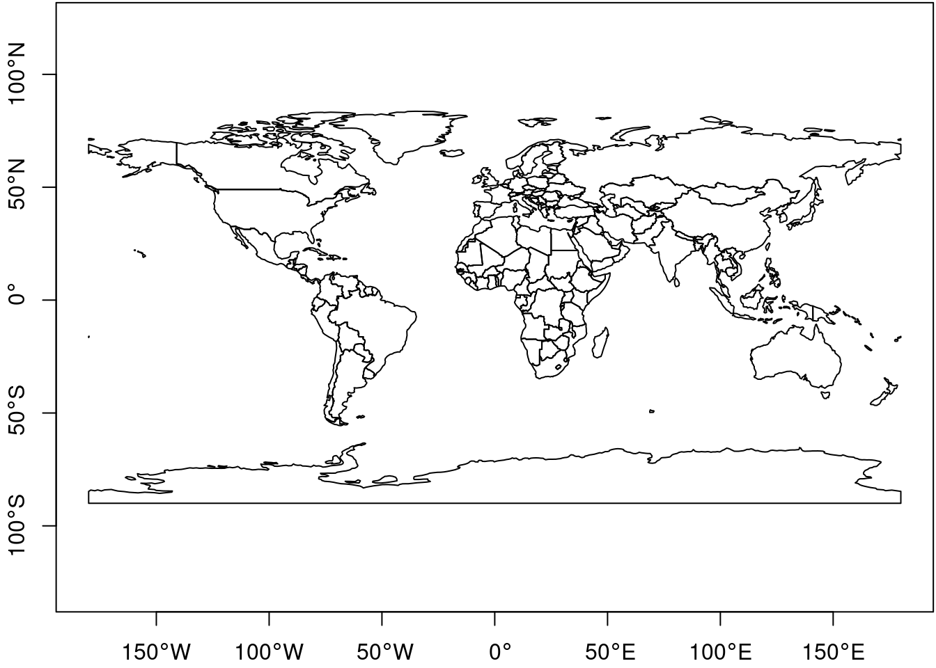
#| fig.cap: "world map, with longitude and latitude map linearly to x and y ([Plate Caree](https://en.wikipedia.org/wiki/Equirectangular_projection))"
library(rnaturalearth)
library(sf)
par(mar = c(2,2,0,0) + .1)
ne_countries() |> st_geometry() |> plot(axes=TRUE)
```
::: {.callout-tip title="What is Statistics"}
... or what *are* statistics?
- statistic: singular; a descriptive measure summarising some data
- statistics: plural; "minimum and maximum are two statistics"
- Statistics: singular; a scientific discipline aiming at modelling data, using probability theory
- where does randomness come from? Design-based vs. model-based
- are parameters random or fixed? Bayesian vs. frequentist
- inference, prediction, simulations
- Typical approach: observation = signal + noise, noise modelled by random variables
:::
### Design-based statistics
In design-based statistics, randomness comes from random sampling. Consider an area $B$, from which we take samples $$z(s),
s \in B,$$ with $s$ a location for instance two-dimensional: $s_i =
\{x_i,y_i\}$. If we select the samples *randomly*, we can consider $S \in B$ a random variable, and $z(S)$ a random sample. Note the randomness in $S$, not in $z$.
Two variables $z(S_1)$ and $z(S_2)$ are *independent* if $S_1$ and $S_2$ are sampled independently. For estimation we need to know the inclusion probabilities, which need to be non-negative for every location.
If inclusion probabilities are constant (simple random sampling; or complete spatial randomness: day 2, point patterns) then we can estimate the mean of $Z(B)$ by the sample mean $$\frac{1}{n}\sum_{j=1}^n
z(s_j).$$ This also predicts the value of a *randomly* chosen observation $z(S)$. It cannot be used to predict the value $z(s_0)$ for a non-randomly chosen location $s_0$; for this we need a model.
### Model-based statistics
Model-based statistics assumes randomness in the measured responses; consider a regression model $y = X\beta + e$, where $e$ is a random variable and as a consequence $y$, the response variable is a random variable. In the spatial context we replace $y$ with $z$, and capitalize it to indicate it is a random variable, and write $$Z(s) = X(s)\beta + e(s)$$ to stress that
- $Z(s)$ is a random function (random variables $Z$ as a function of $s$)
- $X(s)$ is the matrix with covariates, which depend on $s$
- $\beta$ are (spatially) constant coefficients, not depening on $s$
- $e(s)$ is a random function with mean zero and covariance matrix $\Sigma$
In the regression literature this is called a (linear) mixed model, because $e$ is not i.i.d. If $e(s)$ contains an iid component $\epsilon$ we can write this as
$$Z(s) = X(s)\beta + w(s) + \epsilon$$
with $w(s)$ the spatial signal, and $\epsilon$ a noise compenent e.g. due to measurement error.
Predicting $Z(s_0)$ will involve (GLS) estimation of $\beta$, but also prediction of $e(s_0)$ using correlated, nearby observations (day 3: geostatistics).
### Design- or model-based?
- design-based requires a random sample, if that is the case it needs no further assumptions
- model-based requires stationarity assumptions to estimate $\Sigma$
- model-based is typically more effective for interpolation problems
- design-based can be most effective when estimating, e.g. average mapping errors
### Using coordinates as covariates?
- (day 4)
## Spatial statistics: data types
### Point Patterns
- Points (locations) + observation window
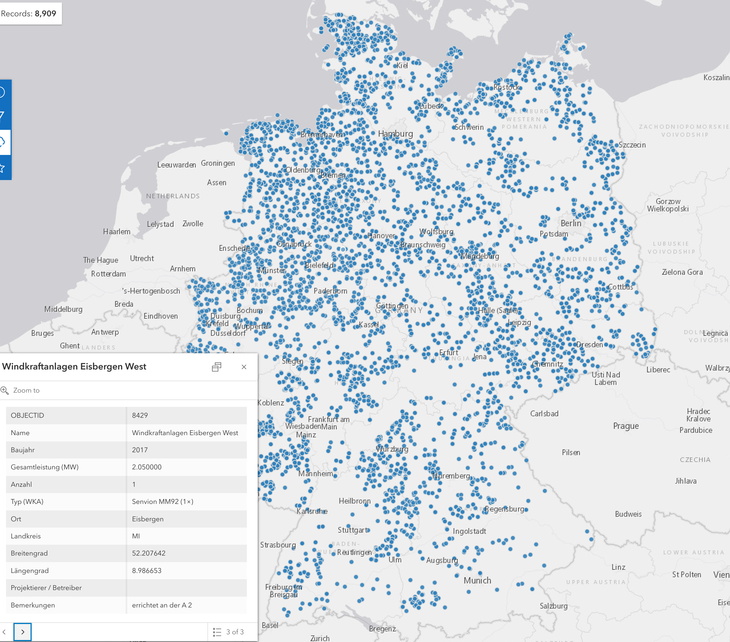
- Example from [here](https://opendata-esri-de.opendata.arcgis.com/datasets/dc6d012f47d94fde99deacc316721f30/explore?location=51.099061%2C10.453852%2C7.45)
```{r fig-gdal-fig-nodetails, echo = FALSE}
#| code-fold: true
#| out.width: '100%'
#| fig.cap: "Wind turbine parks in Germany"
knitr::include_graphics("turbines.png")
```
- The locations contain the information
- Points may have (discrete or continuous) *marks* (attributes)
- The observation window is, apart from the points, *empty*
### Geostatistical data: locations + measured values
```{r}
#| code-fold: true
#| out.width: '100%'
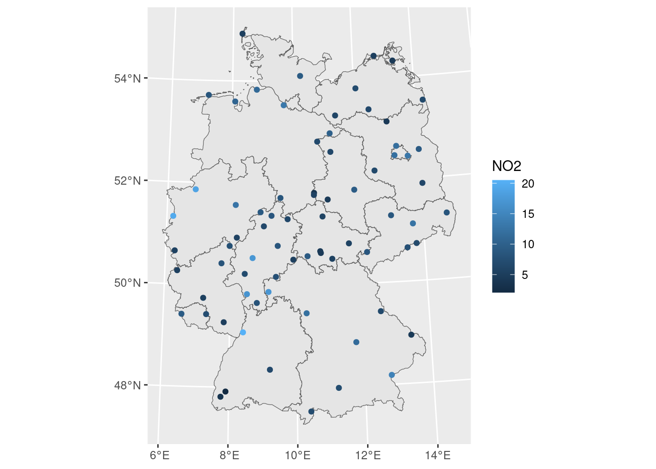
#| fig.cap: "NO2 measurements at rural background stations (EEA)"
library(sf)
no2 <- read.csv(system.file("external/no2.csv",
    package = "gstat"))
crs <- st_crs("EPSG:32632")
st_as_sf(no2, crs = "OGC:CRS84", coords =
    c("station_longitude_deg", "station_latitude_deg")) |>
    st_transform(crs) -> no2.sf
library(ggplot2)
# plot(st_geometry(no2.sf))
"https://github.com/edzer/sdsr/raw/main/data/de_nuts1.gpkg" |>
  read_sf() |>
  st_transform(crs) -> de
ggplot() + geom_sf(data = de) +
    geom_sf(data = no2.sf, mapping = aes(col = NO2))
```
- The value of interest is measured at a set of sample locations
- At other location, this value exists but is *missing*
- The interest is in estimating (predicting) this missing value (interpolation)
- The actual sample locations are not of (primary) interest, the signal is in the measured values
### Areal data
- polygons (or grid cells) + polygon summary values
```{r}
#| code-fold: true
#| out.width: '100%'
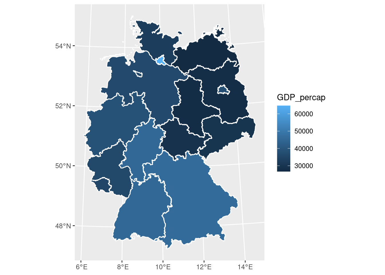
#| fig.cap: "NO2 rural background, average values per NUTS1 region"
# https://en.wikipedia.org/wiki/List_of_NUTS_regions_in_the_European_Union_by_GDP
de$GDP_percap = c(45200, 46100, 37900, 27800, 49700, 64700, 45000, 26700, 36500, 38700, 35700, 35300, 29900, 27400, 32400, 28900)
ggplot() + geom_sf(data = de) +
    geom_sf(data = de, mapping = aes(fill = GDP_percap)) +
    geom_sf(data = st_cast(de, "MULTILINESTRING"), col = 'white')
```
- The polygons contain polygon summary (polygon support) values, not values that are constant throughout the polygon (as in a soil, lithology or land cover map)
- Neighbouring polygons are typically related: spatial correlation
- neighbour-neighbour correlation: Moran's I
- regression models with correlated errors, spatial lag models, CAR models, GMRFs, ...
- see Ch 14-17 of [SDSWR](https://r-spatial.org/book/)
- briefly addressed on Friday
## Data types that received less attention in the spatial statistics literature
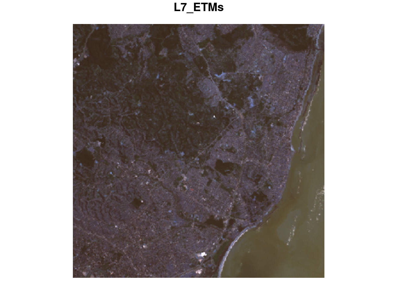
### Image data
```{r}
#| code-fold: true
#| out.width: '100%'
#| fig.cap: "RGB image from a Landsat scene"
library(stars)
plot(L7_ETMs, rgb = 1:3)
```
- are these geostatistical data, or areal data?
- If we identify objects from images, can we see them as point patterns?
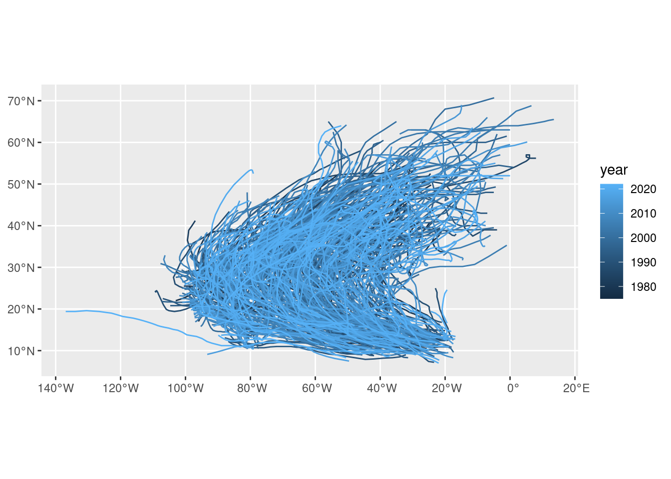
### Tracking data, trajectories
```{r}
#| code-fold: true
#| out.width: '100%'
#| fig.cap: "Storm/hurricane trajectories colored by year"
# from: https://r-spatial.org/r/2017/08/28/nest.html
library(tidyverse)
storms.sf <- storms %>%
st_as_sf(coords = c("long", "lat"), crs = 4326)
storms.sf <- storms.sf %>%
mutate(time = as.POSIXct(paste(paste(year,month,day, sep = "-"),
paste(hour, ":00", sep = "")))) %>%
select(-month, -day, -hour)
storms.nest <- storms.sf %>% group_by(name, year) %>% nest
to_line <- function(tr) st_cast(st_combine(tr), "LINESTRING") %>% .[[1]]
tracks <- storms.nest %>% pull(data) %>% map(to_line) %>% st_sfc(crs = 4326)
storms.tr <- storms.nest %>% select(-data) %>% st_sf(geometry = tracks)
storms.tr %>% ggplot(aes(color = year)) + geom_sf()
```
- A temporal snapshot (time slice) of a set of moving things forms a point pattern
- We often analyse trajectories by
- estimating densities, for space-time blocks, per individual or together
- analysing interactions (alibi problem, mating animals, home range, UDF etc)
## Checklist if you have spatial data
- Do you have the spatial coordinates of your data?
- Are the coordinates Earth-bound?
- If yes, do you have the coordinate reference system of them?
- What is the support (physical size) of your observations?
- Were the data obtained by random sampling, and if yes, do you have sampling weights?
- Do you know the *extent* ($B$) from which your data were sampled, or collected?
## Exercises
- What is the coordinate reference system of the `ne_countries()` dataset, imported above?
- Look up the "Equidistant Cylindrical (Plate Carrée)" projection on the <https://proj.org> website.
- Why is this projection called *The simplest of all projections*?
- Project `ne_countries` to Plate Carrée, and plot it with `axes=TRUE`. What has changed? (Hint: `st_crs()` accepts a *proj string* to define a coordinate reference system (CRS); `st_transform()` transforms a dataset to a new CRS.)
- Project the same dataset to Eckert IV projection. What has changed?
- Also try plotting this dataset after transforming it to an orthographic projection with `+proj=ortho`; what went wrong?
[Link to Answers](day1_ex.html)
## Further reading
- Ripley, B. 1981. Spatial Statistics. Wiley.
- Cressie, N. 1993. Statistics for Spatial Data. Wiley.
- Cochran, W.G. 1977. Sampling Techniques. Wiley.
- references in [Spatial Data Science; with applications in R](https://r-spatial.org/book/)