library(dplyr)
#
# Attaching package: 'dplyr'
# The following objects are masked from 'package:stats':
#
#     filter, lag
# The following objects are masked from 'package:base':
#
#     intersect, setdiff, setequal, union
library(sf)
# Linking to GEOS 3.12.2, GDAL 3.11.4, PROJ 9.4.1; sf_use_s2() is
# TRUE
crs <- st_crs("EPSG:32632") # a csv doesn't carry a CRS!
no2 <- read.csv(system.file("external/no2.csv",
    package = "gstat"))
no2 |> rename(x = station_longitude_deg, y = station_latitude_deg)  |>
  st_as_sf(crs = "OGC:CRS84", coords =
    c("x", "y"), remove = FALSE) |>
    st_transform(crs) -> no2.sf
# we need to reassign x and y:
cc = st_coordinates(no2.sf)
no2.sf$x = cc[,1]
no2.sf$y = cc[,2]
head(no2.sf)
# Simple feature collection with 6 features and 21 fields
# Geometry type: POINT
# Dimension:     XY
# Bounding box:  xmin: 495000 ymin: 5320000 xmax: 816000 ymax: 5930000
# Projected CRS: WGS 84 / UTM zone 32N
#   station_european_code station_local_code country_iso_code
# 1               DENI063            DENI063               DE
# 2               DEBY109            DEBY109               DE
# 3               DEBE056            DEBE056               DE
# 4               DEBE062            DEBE062               DE
# 5               DEBE032            DEBE032               DE
# 6               DEHE046            DEHE046               DE
#   country_name                station_name station_start_date
# 1      Germany                  Altes Land         1999-02-11
# 2      Germany          Andechs/Rothenfeld         2003-04-17
# 3      Germany           B Friedrichshagen         1994-02-01
# 4      Germany B Frohnau, Funkturm (3.5 m)         1996-02-01
# 5      Germany         B Grunewald (3.5 m)         1986-10-01
# 6      Germany                 Bad Arolsen         1999-05-11
#   station_end_date type_of_station station_ozone_classification
# 1               NA      Background                        rural
# 2               NA      Background                        rural
# 3               NA      Background                        rural
# 4               NA      Background                        rural
# 5               NA      Background                        rural
# 6               NA      Background                        rural
#   station_type_of_area station_subcat_rural_back street_type      x
# 1                rural                   unknown             545414
# 2                rural                  regional             665711
# 3                rural                 near city             815741
# 4                rural                 near city             790544
# 5                rural                 near city             786923
# 6                rural                   unknown             495007
#         y station_altitude          station_city lau_level1_code
# 1 5930802                3                                    NA
# 2 5315213              700                                    NA
# 3 5820995               35                                    NA
# 4 5842367               50                BERLIN              NA
# 5 5822067               50                BERLIN              NA
# 6 5697747              343 BAD AROLSEN/KOHLGRUND              NA
#   lau_level2_code    lau_level2_name EMEP_station   NO2
# 1         3359028               Jork           no 13.10
# 2         9188117            Andechs           no  7.14
# 3        11000000      Berlin, Stadt           no 12.80
# 4        11000000      Berlin, Stadt           no 11.83
# 5        11000000      Berlin, Stadt           no 11.98
# 6         6635002 Bad Arolsen, Stadt           no  8.94
#                 geometry
# 1 POINT (545414 5930802)
# 2 POINT (665711 5315213)
# 3 POINT (815741 5820995)
# 4 POINT (790544 5842367)
# 5 POINT (786923 5822067)
# 6 POINT (495007 5697747)
"https://github.com/edzer/sdsr/raw/main/data/de_nuts1.gpkg" |>
  read_sf() |>
st_transform(crs) -> de4 Machine Learning methods applied to spatial data
Learning goals
Reading materials
From Spatial Data Science: with applications in R:
- Section 10.1: Mapping with non-spatial regression and ML models (you already read this)
From the stars vignettes:
- Statistical modelling with stars objects
Area of Applicability:
- this CAST vignette
- Machine learning-based global maps of ecological variables and the challenge of assessing them
TipSummary
- Intro to prediction with R
- (functions of) Spatial coordinates as predictors
- Spatially correlated residuals
- Area of applicability
- RandomForestsGLS: Random forests for dependent data
Summary
- Data: coverages as predictors
- Pitfalls: independence, known predictors, clustered data, different support / spatial unalignment
- Model assessment and transferrability: cross validation strategies, area of applicability
- RandomForestsGLS
4.1 Spatial coordinates as predictor
We’ll rename coordinates to x and y:
library(stars)
# Loading required package: abind
g2 = st_as_stars(st_bbox(de))
g3 = st_crop(g2, de)
g4 = st_rasterize(de, g3)
g4$ID_1[g4$ID_1 == 758] = NA
g4$ID1 = as.factor(g4$ID_1) # now a factor:
plot(g4["ID1"], reset = FALSE)
plot(st_geometry(no2.sf), add = TRUE, col = 'green')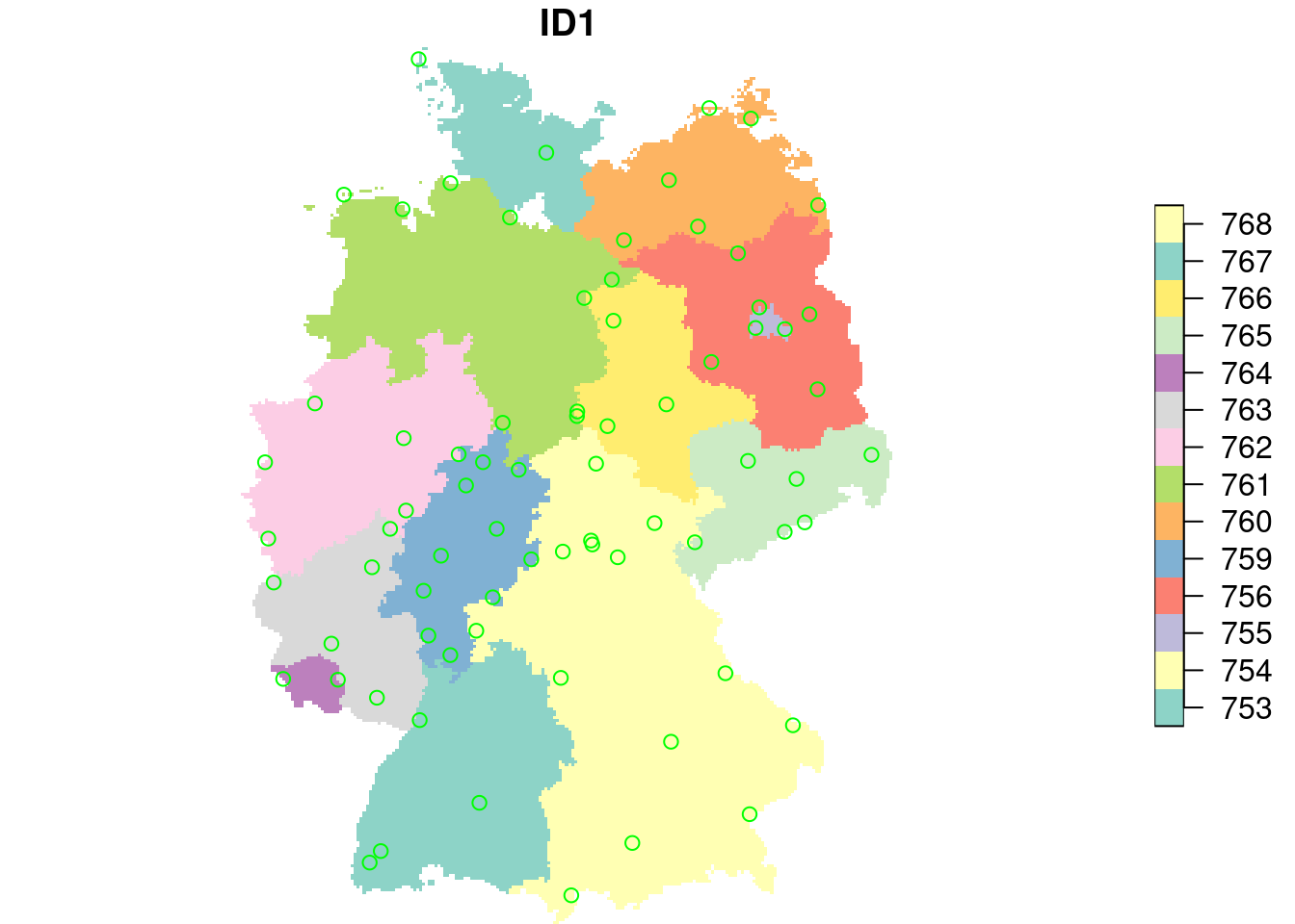
no2.sf$ID1 = st_extract(g4, no2.sf)$ID1
no2.sf$ID1 |> summary()
#  753  754  755  756  759  760  761  762  763  764  765  766  767
#    4    8    3    4   10    6    6    6    6    1    6    5    1
#  768 NA's
#    6    2
Simple ANOVA type predictor:
lm1 = lm(NO2~ID1, no2.sf)
summary(lm1)
#
# Call:
# lm(formula = NO2 ~ ID1, data = no2.sf)
#
# Residuals:
#    Min     1Q Median     3Q    Max
# -6.324 -1.599 -0.311  0.859 12.358
#
# Coefficients:
#             Estimate Std. Error t value Pr(>|t|)
# (Intercept)    8.136      1.873    4.34  5.7e-05 ***
# ID1754         1.883      2.294    0.82     0.41
# ID1755         4.068      2.861    1.42     0.16
# ID1756        -1.593      2.649   -0.60     0.55
# ID1759         1.015      2.216    0.46     0.65
# ID1760        -2.215      2.418   -0.92     0.36
# ID1761         1.353      2.418    0.56     0.58
# ID1762         3.697      2.418    1.53     0.13
# ID1763        -1.724      2.418   -0.71     0.48
# ID1764         1.091      4.188    0.26     0.80
# ID1765         0.591      2.418    0.24     0.81
# ID1766        -2.282      2.513   -0.91     0.37
# ID1767         1.024      4.188    0.24     0.81
# ID1768        -2.358      2.418   -0.98     0.33
# ---
# Signif. codes:  0 '***' 0.001 '**' 0.01 '*' 0.05 '.' 0.1 ' ' 1
#
# Residual standard error: 3.75 on 58 degrees of freedom
#   (2 observations deleted due to missingness)
# Multiple R-squared:  0.268,   Adjusted R-squared:  0.104
# F-statistic: 1.63 on 13 and 58 DF,  p-value: 0.102
g4$NO2_aov = predict(lm1, as.data.frame(g4))
plot(g4["NO2_aov"], breaks = "equal", reset = FALSE)
plot(st_cast(st_geometry(de), "MULTILINESTRING"), add = TRUE, col = 'green')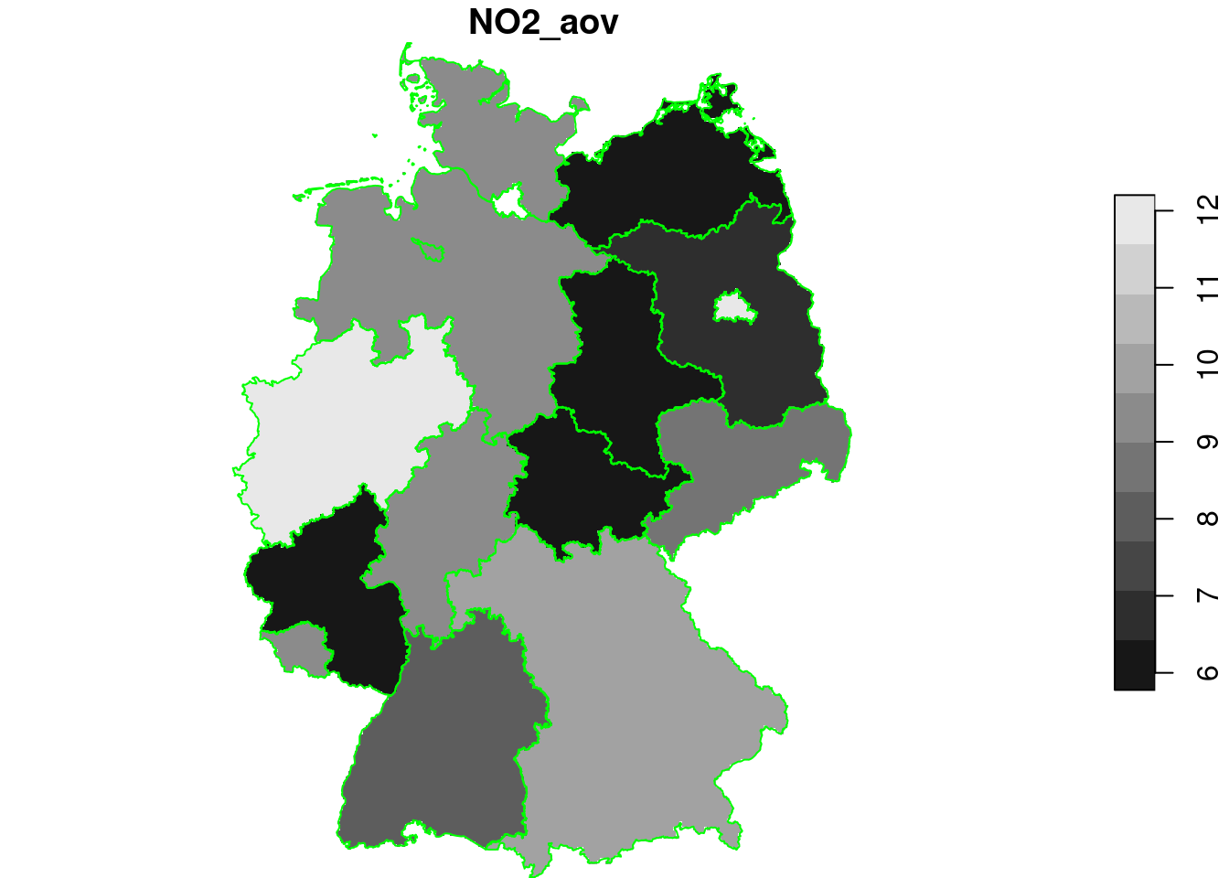
Simple linear models in coordinates: trend surfaces
lm2 = lm(NO2~x+y, no2.sf)
summary(lm2)
#
# Call:
# lm(formula = NO2 ~ x + y, data = no2.sf)
#
# Residuals:
#    Min     1Q Median     3Q    Max
# -6.880 -2.634 -0.991  1.431 11.660
#
# Coefficients:
#              Estimate Std. Error t value Pr(>|t|)
# (Intercept)  9.47e+00   1.36e+01    0.70     0.49
# x           -3.66e-06   3.00e-06   -1.22     0.23
# y            1.91e-07   2.45e-06    0.08     0.94
#
# Residual standard error: 3.95 on 71 degrees of freedom
# Multiple R-squared:  0.0212,  Adjusted R-squared:  -0.00637
# F-statistic: 0.769 on 2 and 71 DF,  p-value: 0.467
cc = st_coordinates(g4)
g4$x = cc[,1]
g4$y = cc[,2]
g4$NO2_lm2 = predict(lm2, g4)
plot(g4["NO2_lm2"], breaks = "equal", reset = FALSE, main = "1st order polynomial")
plot(st_cast(st_geometry(de), "MULTILINESTRING"), add = TRUE, col = 'green')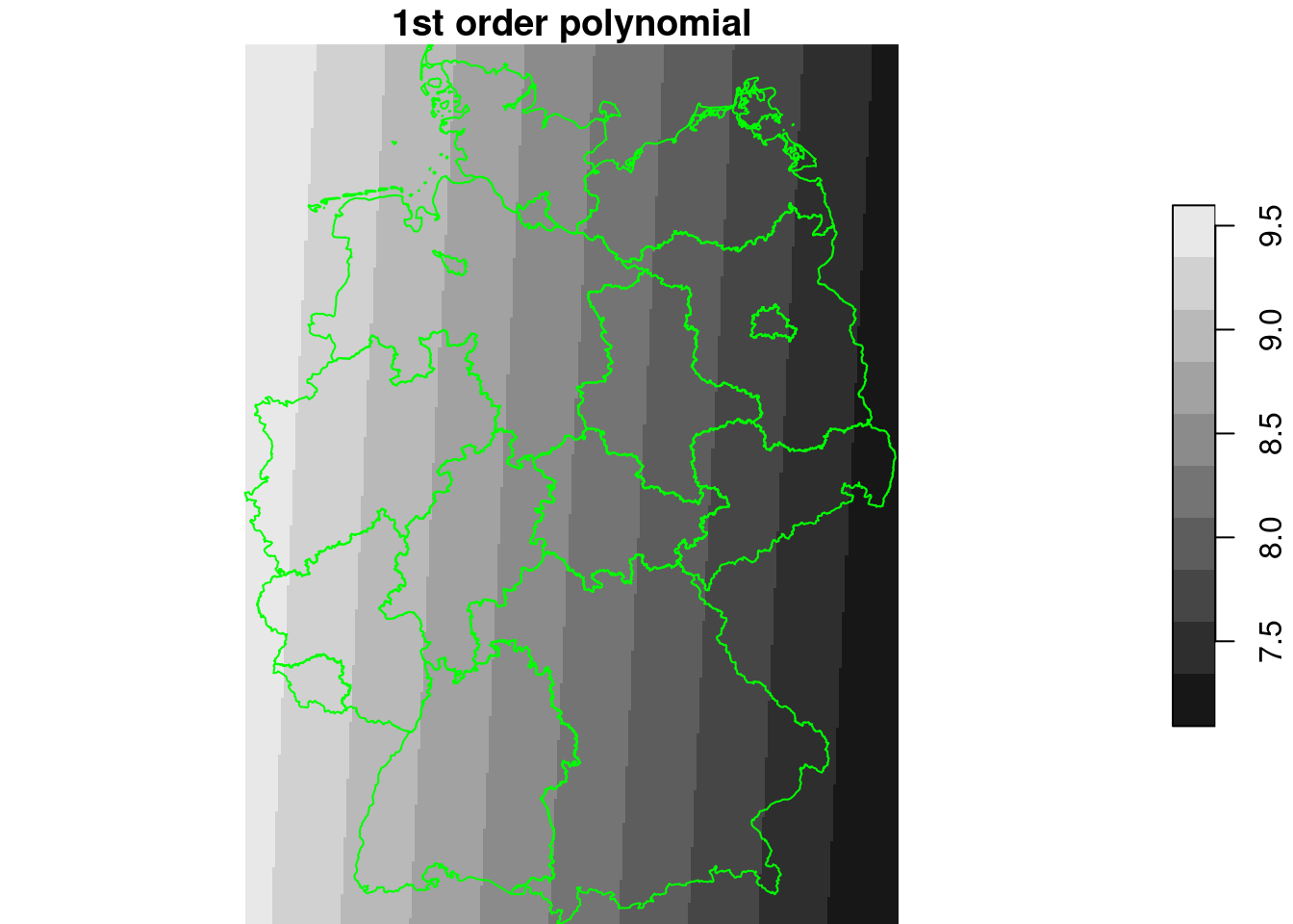
lm3 = lm(NO2~x+y+I(x^2)+I(y^2)+I(x*y), no2.sf)
summary(lm3)
#
# Call:
# lm(formula = NO2 ~ x + y + I(x^2) + I(y^2) + I(x * y), data = no2.sf)
#
# Residuals:
#    Min     1Q Median     3Q    Max
# -5.480 -2.583 -0.585  1.523 12.750
#
# Coefficients:
#              Estimate Std. Error t value Pr(>|t|)
# (Intercept) -4.24e+02   3.27e+02   -1.30    0.199
# x            1.34e-04   9.13e-05    1.47    0.147
# y            1.39e-04   1.14e-04    1.21    0.230
# I(x^2)       2.52e-11   1.91e-11    1.32    0.190
# I(y^2)      -1.06e-11   1.01e-11   -1.05    0.296
# I(x * y)    -2.96e-11   1.65e-11   -1.79    0.077 .
# ---
# Signif. codes:  0 '***' 0.001 '**' 0.01 '*' 0.05 '.' 0.1 ' ' 1
#
# Residual standard error: 3.87 on 68 degrees of freedom
# Multiple R-squared:  0.0972,  Adjusted R-squared:  0.0308
# F-statistic: 1.46 on 5 and 68 DF,  p-value: 0.213
g4$NO2_lm3 = predict(lm3, g4)
plot(g4["NO2_lm3"], breaks = "equal", reset = FALSE, main = "2nd order polynomial")
plot(st_cast(st_geometry(de), "MULTILINESTRING"), add = TRUE, col = 'green')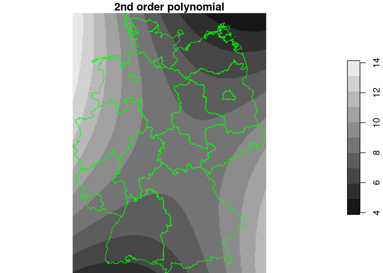
lm4 = lm(NO2~x+y+I(x^2)+I(y^2)+I(x*y)+I(x^3)+I(x^2*y)+I(x*y^2)+I(y^3), no2.sf)
summary(lm4)
#
# Call:
# lm(formula = NO2 ~ x + y + I(x^2) + I(y^2) + I(x * y) + I(x^3) +
#     I(x^2 * y) + I(x * y^2) + I(y^3), data = no2.sf)
#
# Residuals:
#    Min     1Q Median     3Q    Max
# -5.285 -2.582 -0.796  2.074 12.693
#
# Coefficients:
#              Estimate Std. Error t value Pr(>|t|)
# (Intercept)  3.38e+03   9.12e+03    0.37    0.712
# x            5.15e-03   2.50e-03    2.06    0.043 *
# y           -2.40e-03   4.84e-03   -0.49    0.622
# I(x^2)      -1.19e-09   7.46e-10   -1.60    0.115
# I(y^2)       5.15e-10   8.59e-10    0.60    0.551
# I(x * y)    -1.54e-09   8.57e-10   -1.80    0.077 .
# I(x^3)       1.13e-16   1.31e-16    0.86    0.394
# I(x^2 * y)   1.80e-16   1.38e-16    1.30    0.197
# I(x * y^2)   1.14e-16   7.75e-17    1.47    0.146
# I(y^3)      -3.49e-17   5.10e-17   -0.68    0.496
# ---
# Signif. codes:  0 '***' 0.001 '**' 0.01 '*' 0.05 '.' 0.1 ' ' 1
#
# Residual standard error: 3.82 on 64 degrees of freedom
# Multiple R-squared:  0.173,   Adjusted R-squared:  0.0572
# F-statistic: 1.49 on 9 and 64 DF,  p-value: 0.17
g4$NO2_lm4 = predict(lm4, g4)
plot(g4["NO2_lm4"], breaks = "equal", reset = FALSE, main = "3rd order polynomial")
plot(st_cast(st_geometry(de), "MULTILINESTRING"), add = TRUE, col = 'green')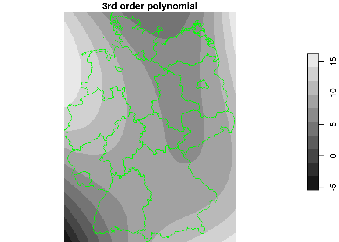
regression tree
library(rpart)
tree = rpart(NO2~., as.data.frame(no2.sf)[c("NO2", "x", "y")])
g4$tree = predict(tree, as.data.frame(g4))
plot(g4["tree"], breaks = "equal", reset = FALSE, main = "regression tree")
plot(st_cast(st_geometry(de), "MULTILINESTRING"), add = TRUE, col = 'green')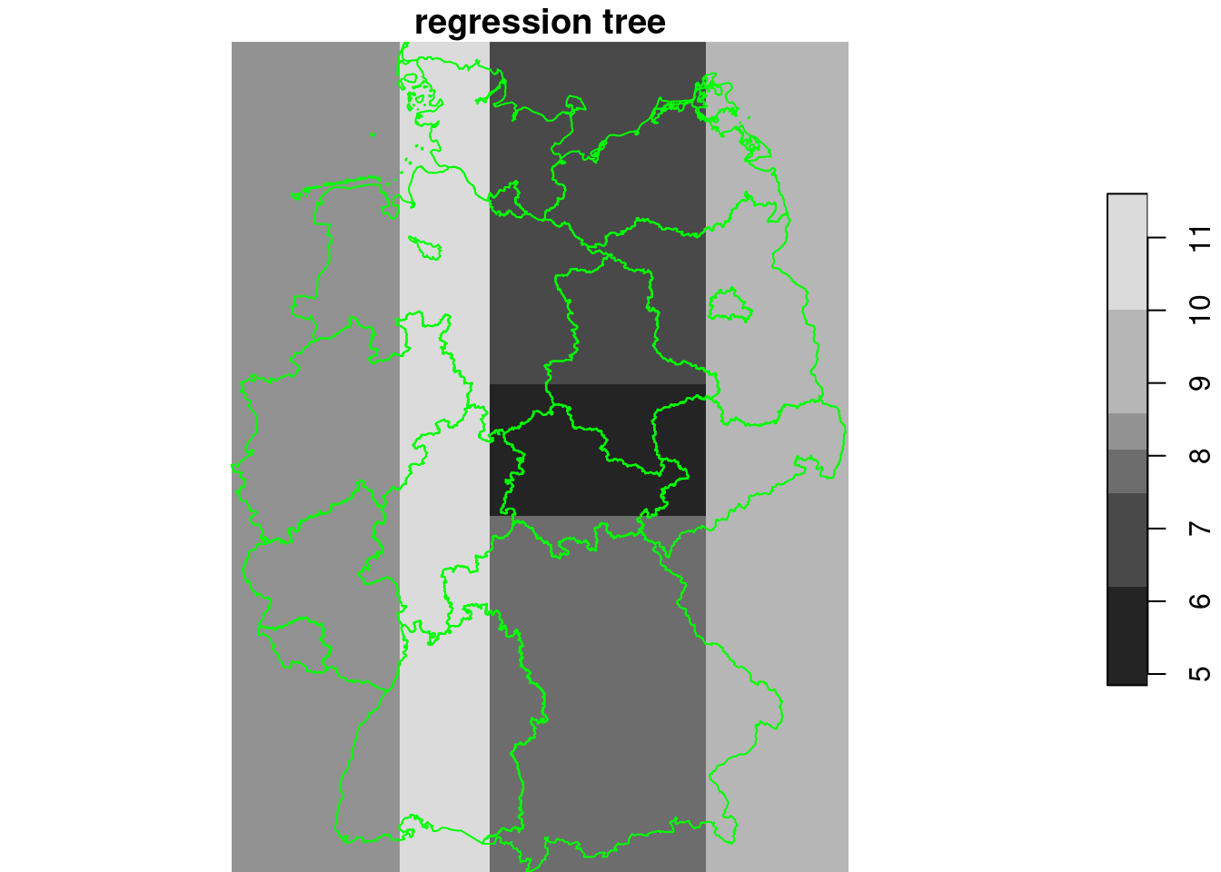
Random forest
library(randomForest)
# randomForest 4.7-1.2
# Type rfNews() to see new features/changes/bug fixes.
#
# Attaching package: 'randomForest'
# The following object is masked from 'package:dplyr':
#
#     combine
rf = randomForest(NO2~., as.data.frame(no2.sf)[c("NO2", "x", "y")])
g4$rf = predict(rf, as.data.frame(g4))
plot(g4["rf"], breaks = "equal", reset = FALSE, main = "random forest")
plot(st_cast(st_geometry(de), "MULTILINESTRING"), add = TRUE, col = 'green')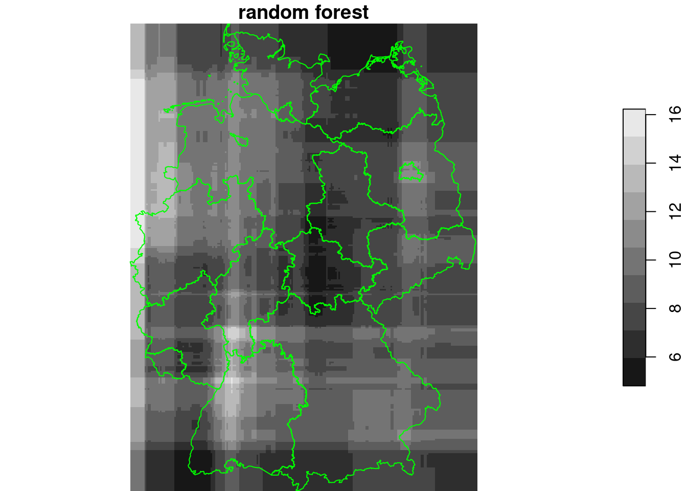
Rotated coordinates:
library(randomForest)
no2.sf$x1 = no2.sf$x + no2.sf$y
no2.sf$y1 = no2.sf$x - no2.sf$y
rf = randomForest(NO2~., as.data.frame(no2.sf)[c("NO2", "x1", "y1")])
g4$x1 = g4$x + g4$y
g4$y1 = g4$x - g4$y
g4$rf_rot = predict(rf, as.data.frame(g4))
plot(g4["rf_rot"], breaks = "equal", reset = FALSE, main = "random forest")
plot(st_cast(st_geometry(de), "MULTILINESTRING"), add = TRUE, col = 'green')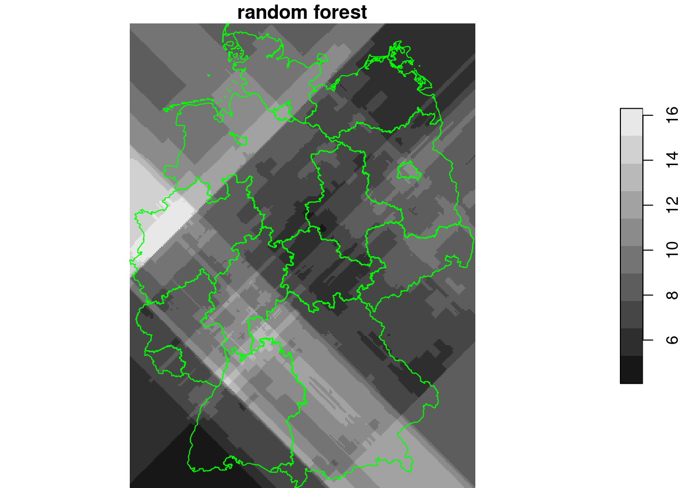
Using distance variables
st_bbox(de) |> st_as_sfc() |> st_cast("POINT") -> pts
pts = c(pts[1:4], st_centroid(st_geometry(de)))
d = st_distance(st_as_sfc(g4, as_points = TRUE), pts)
for (i in seq_len(ncol(d))) {
    g4[[ paste0("d_", i) ]] = d[,i]
}
e = st_extract(g4, no2.sf)
for (i in seq_len(ncol(d))) {
    no2.sf[[ paste0("d_", i) ]] = e[[16+i]]
}
(n = names(g4))
#  [1] "ID_0"       "ID_1"       "Shape_Leng" "Shape_Area"
#  [5] "ID1"        "NO2_aov"    "x"          "y"
#  [9] "NO2_lm2"    "NO2_lm3"    "NO2_lm4"    "tree"
# [13] "rf"         "x1"         "y1"         "rf_rot"
# [17] "d_1"        "d_2"        "d_3"        "d_4"
# [21] "d_5"        "d_6"        "d_7"        "d_8"
# [25] "d_9"        "d_10"       "d_11"       "d_12"
# [29] "d_13"       "d_14"       "d_15"       "d_16"
# [33] "d_17"       "d_18"       "d_19"       "d_20"
plot(merge(g4[grepl("d_", n)]))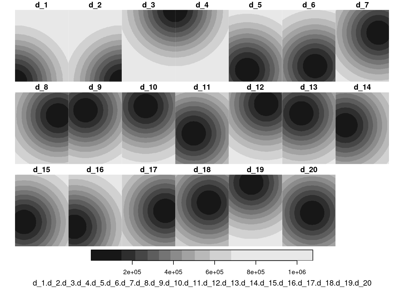
library(randomForest)
rf = randomForest(NO2~., as.data.frame(no2.sf)[c("NO2", n[grepl("d_", n)])])
g4$rf_d = predict(rf, as.data.frame(g4))
plot(g4["rf_d"], breaks = "equal", reset = FALSE, main = "random forest")
plot(st_cast(st_geometry(de), "MULTILINESTRING"), add = TRUE, col = 'green')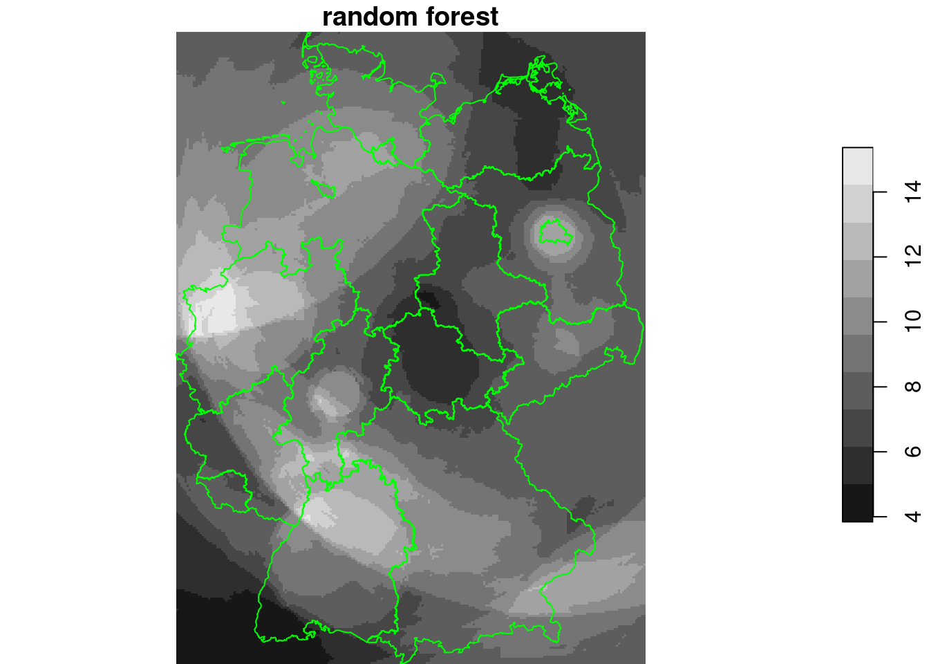
Adding many more distance variables
# sample 200 points as centers for distance function, using regular sampling
pts = st_sample(de, 200, type = "regular")
# compute distances between these 200 pts and all grid cell centers
d = st_distance(st_as_sfc(g4, as_points = TRUE), pts)
# add these distance fields to the g4 stars object:
for (i in seq_len(ncol(d))) {
    g4[[ paste0("d_", i) ]] = d[,i]
}
# extract distance field values at no2.sf station locations:
e = st_extract(g4, no2.sf)
# add these as columns to no2.sf:
for (i in seq_len(ncol(d))) {
    no2.sf[[ paste0("d_", i) ]] = e[[16+i]]
}
(n = names(g4))
#   [1] "ID_0"       "ID_1"       "Shape_Leng" "Shape_Area"
#   [5] "ID1"        "NO2_aov"    "x"          "y"
#   [9] "NO2_lm2"    "NO2_lm3"    "NO2_lm4"    "tree"
#  [13] "rf"         "x1"         "y1"         "rf_rot"
#  [17] "d_1"        "d_2"        "d_3"        "d_4"
#  [21] "d_5"        "d_6"        "d_7"        "d_8"
#  [25] "d_9"        "d_10"       "d_11"       "d_12"
#  [29] "d_13"       "d_14"       "d_15"       "d_16"
#  [33] "d_17"       "d_18"       "d_19"       "d_20"
#  [37] "rf_d"       "d_21"       "d_22"       "d_23"
#  [41] "d_24"       "d_25"       "d_26"       "d_27"
#  [45] "d_28"       "d_29"       "d_30"       "d_31"
#  [49] "d_32"       "d_33"       "d_34"       "d_35"
#  [53] "d_36"       "d_37"       "d_38"       "d_39"
#  [57] "d_40"       "d_41"       "d_42"       "d_43"
#  [61] "d_44"       "d_45"       "d_46"       "d_47"
#  [65] "d_48"       "d_49"       "d_50"       "d_51"
#  [69] "d_52"       "d_53"       "d_54"       "d_55"
#  [73] "d_56"       "d_57"       "d_58"       "d_59"
#  [77] "d_60"       "d_61"       "d_62"       "d_63"
#  [81] "d_64"       "d_65"       "d_66"       "d_67"
#  [85] "d_68"       "d_69"       "d_70"       "d_71"
#  [89] "d_72"       "d_73"       "d_74"       "d_75"
#  [93] "d_76"       "d_77"       "d_78"       "d_79"
#  [97] "d_80"       "d_81"       "d_82"       "d_83"
# [101] "d_84"       "d_85"       "d_86"       "d_87"
# [105] "d_88"       "d_89"       "d_90"       "d_91"
# [109] "d_92"       "d_93"       "d_94"       "d_95"
# [113] "d_96"       "d_97"       "d_98"       "d_99"
# [117] "d_100"      "d_101"      "d_102"      "d_103"
# [121] "d_104"      "d_105"      "d_106"      "d_107"
# [125] "d_108"      "d_109"      "d_110"      "d_111"
# [129] "d_112"      "d_113"      "d_114"      "d_115"
# [133] "d_116"      "d_117"      "d_118"      "d_119"
# [137] "d_120"      "d_121"      "d_122"      "d_123"
# [141] "d_124"      "d_125"      "d_126"      "d_127"
# [145] "d_128"      "d_129"      "d_130"      "d_131"
# [149] "d_132"      "d_133"      "d_134"      "d_135"
# [153] "d_136"      "d_137"      "d_138"      "d_139"
# [157] "d_140"      "d_141"      "d_142"      "d_143"
# [161] "d_144"      "d_145"      "d_146"      "d_147"
# [165] "d_148"      "d_149"      "d_150"      "d_151"
# [169] "d_152"      "d_153"      "d_154"      "d_155"
# [173] "d_156"      "d_157"      "d_158"      "d_159"
# [177] "d_160"      "d_161"      "d_162"      "d_163"
# [181] "d_164"      "d_165"      "d_166"      "d_167"
# [185] "d_168"      "d_169"      "d_170"      "d_171"
# [189] "d_172"      "d_173"      "d_174"      "d_175"
# [193] "d_176"      "d_177"      "d_178"      "d_179"
# [197] "d_180"      "d_181"      "d_182"      "d_183"
# [201] "d_184"      "d_185"      "d_186"      "d_187"
# [205] "d_188"      "d_189"      "d_190"      "d_191"
# [209] "d_192"      "d_193"      "d_194"      "d_195"
# [213] "d_196"      "d_197"      "d_198"      "d_199"
# [217] "d_200"      "d_201"      "d_202"      "d_203"
# [221] "d_204"      "d_205"      "d_206"
rf = randomForest(NO2~., as.data.frame(no2.sf)[c("NO2", n[grepl("d_", n)])])
g4$rf_dm = predict(rf, as.data.frame(g4))
plot(g4["rf_dm"], breaks = "equal", reset = FALSE, main = "random forest")
plot(st_cast(st_geometry(de), "MULTILINESTRING"), add = TRUE, col = 'green')
plot(st_geometry(no2.sf), add = TRUE, col = 'orange')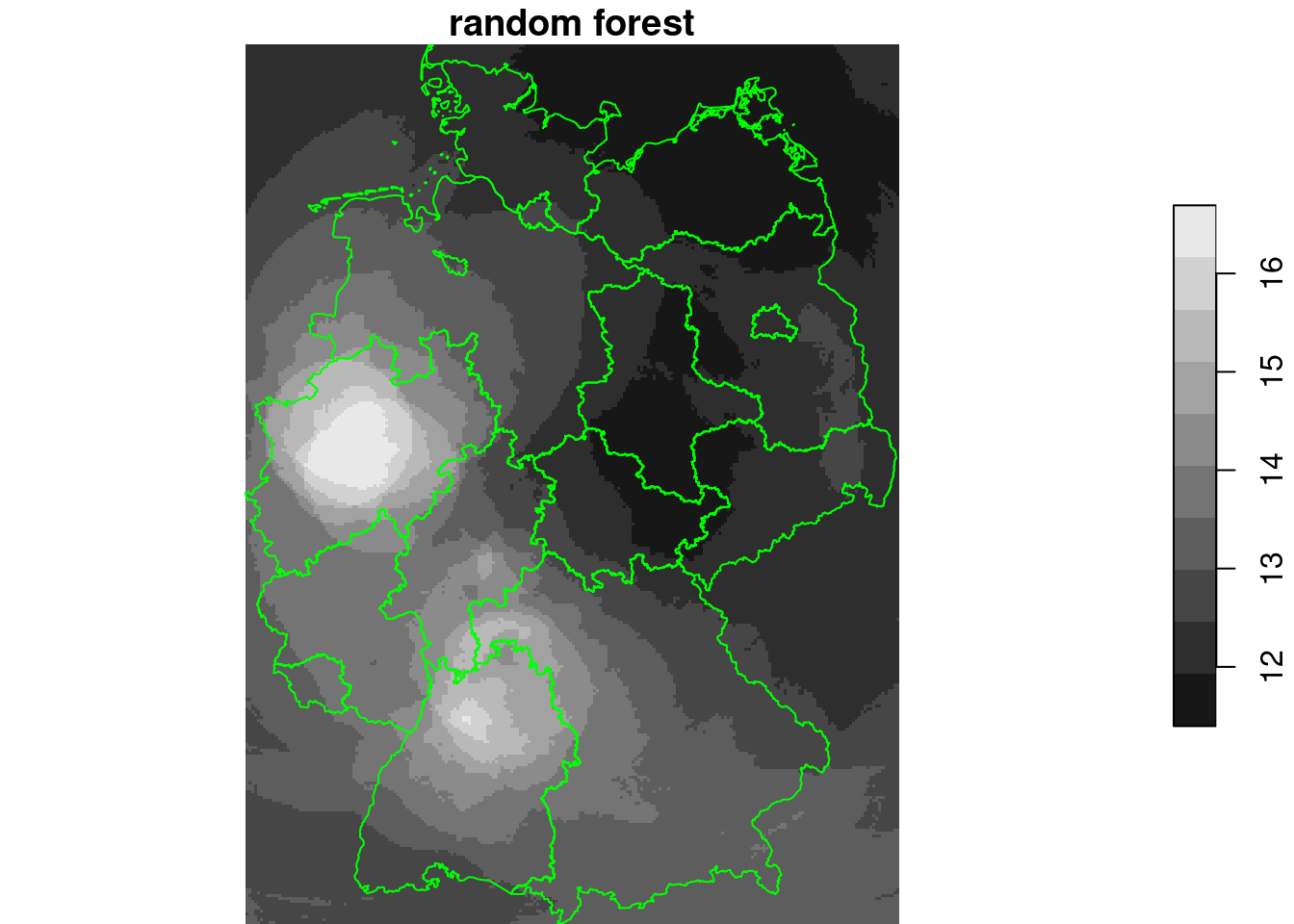
Further approaches:
- using linear regression on Gaussian kernel basis functions, \(\exp(-h^2)\)
- using splines in \(x\) and \(y\), with a given degree of smoothing (or effective degrees of freedom)
- using additional, non-distance/coordinate functions as base function(s)
- provided they are available “everywhere” (as coverage)
- examples: elevation, bioclimatic variables, (values derived from) satellite imagery bands
4.2 Exercises
- Discuss how will a predicted surface look like when instead of (linear functions of) coordinates, the variable elevation is used (e.g. to predict average temperatures)?
- What will be the value range, approximately, of the resulting predicted values, when a first order linear model is used?
- Discuss How would you assess whether residuals from your fitted model are spatially correlated?
- Compute such a variogram for the residuals of the last random forets model shown, and consider whether residual spatial correlation is present
- Discuss: Does resampling using random partitioning (as is done in random forest) implicitly assume that observations are independent?
Example from CAST / caret
library(CAST)
library(caret)
# Loading required package: ggplot2
#
# Attaching package: 'ggplot2'
# The following object is masked from 'package:randomForest':
#
#     margin
# Loading required package: lattice
data(splotdata)
class(splotdata)
# [1] "sf"         "data.frame"
r = read_stars(system.file("extdata/predictors_chile.tif",
                           package = "CAST"))
x = st_drop_geometry(splotdata)[,6:16]
y = splotdata$Species_richness
tr = train(x, y) # chooses a random forest by default
predict(split(r), tr) |> plot()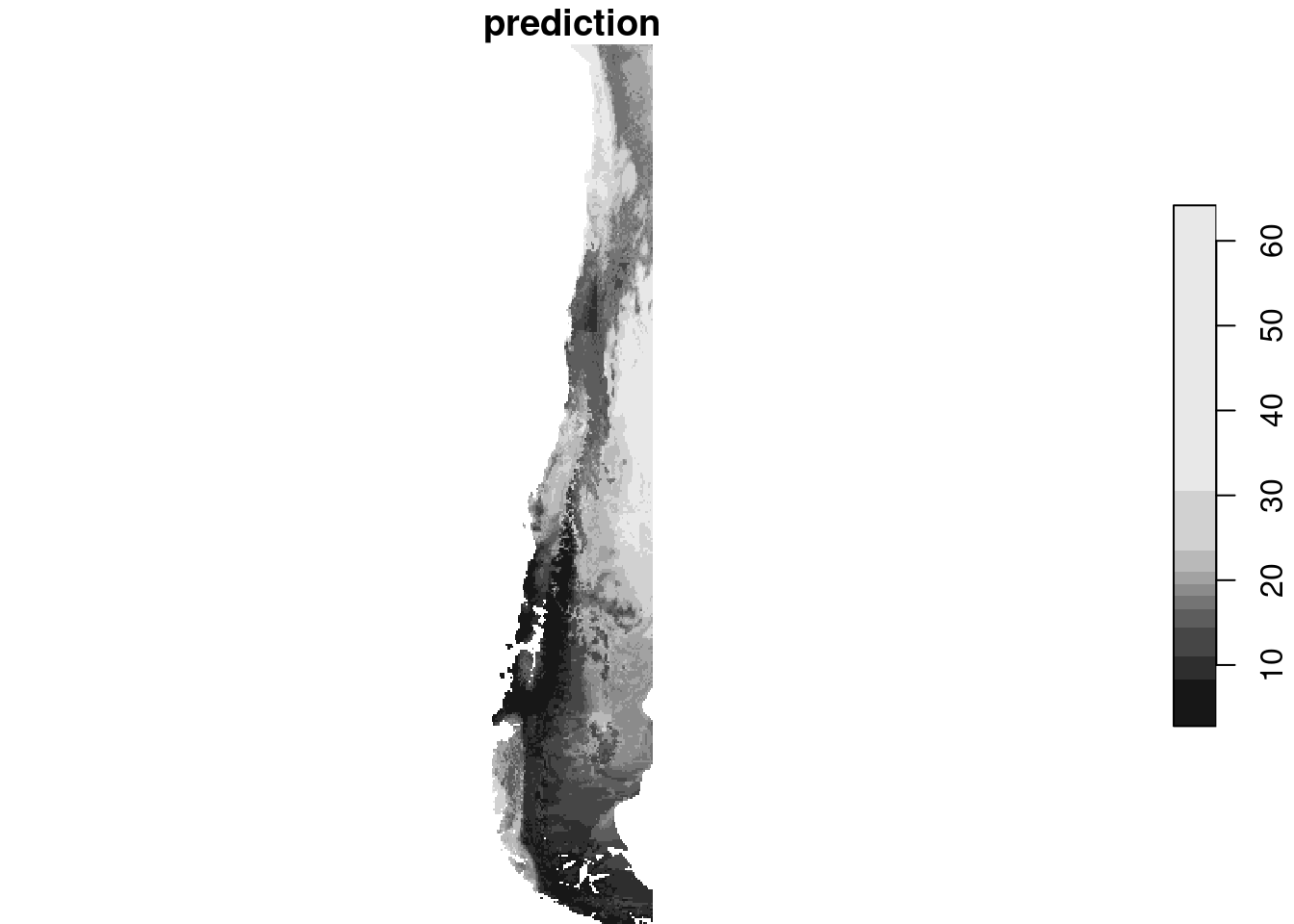
Clustered data?
plot(r[,,,1], reset = FALSE)
plot(st_geometry(splotdata), add = TRUE, col = 'green')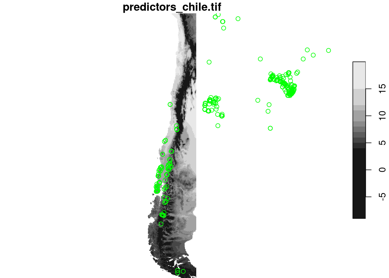
4.3 Cross validation: random or spatially blocked?
4.4 Transferrability of models: “area of applicability”
Explained here;
aoa <- aoa(r, tr, verbose = FALSE)
# note: Either no model was given or no CV was used for model training. The DI threshold is therefore based on all training data
plot(aoa)
# Warning: `aes_string()` was deprecated in ggplot2 3.0.0.
# ℹ Please use tidy evaluation idioms with `aes()`.
# ℹ See also `vignette("ggplot2-in-packages")` for more information.
# ℹ The deprecated feature was likely used in the CAST package.
#   Please report the issue at
#   <https://github.com/HannaMeyer/CAST/issues/>.
# Warning: Removed 395 rows containing non-finite outside the scale range
# (`stat_density()`).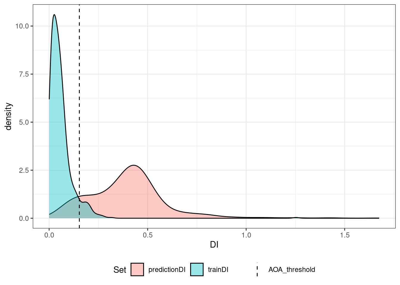
plot(aoa$DI)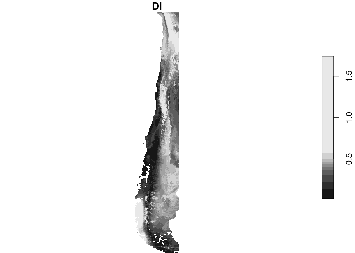
plot(aoa$AOA)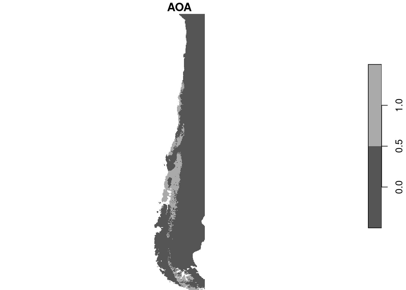
4.5 ML methods for Spatially Dependent Data
R package RandomForestGLS!
Combines the good parts of RF and Gaussian processes, in a very smart way! (final paper, paywalled, here). The discussion on variable selection / variable importance under spatial correlated residuals is worth reading.
library(RandomForestsGLS)
cc = st_coordinates(splotdata)
if (file.exists("rfgls.rda")) {
    load("rfgls.rda") # loads rfgls
} else {
     rfgls = RFGLS_estimate_spatial(cc, as.double(y), x) # takes a while
}
cc_pr = st_coordinates(split(r))
head(as.data.frame(split(r)))
#       x     y bio_1 bio_4 bio_5 bio_6 bio_8 bio_9 bio_12 bio_13
# 1 -75.6 -17.6    NA    NA    NA    NA    NA    NA     NA     NA
# 2 -75.5 -17.6    NA    NA    NA    NA    NA    NA     NA     NA
# 3 -75.5 -17.6    NA    NA    NA    NA    NA    NA     NA     NA
# 4 -75.4 -17.6    NA    NA    NA    NA    NA    NA     NA     NA
# 5 -75.3 -17.6    NA    NA    NA    NA    NA    NA     NA     NA
# 6 -75.2 -17.6    NA    NA    NA    NA    NA    NA     NA     NA
#   bio_14 bio_15 elev
# 1     NA     NA   NA
# 2     NA     NA   NA
# 3     NA     NA   NA
# 4     NA     NA   NA
# 5     NA     NA   NA
# 6     NA     NA   NA
pr = RFGLS_predict_spatial(rfgls, as.matrix(cc_pr), as.data.frame(split(r))[-(1:2)])
# Warning in BRISC_estimation(coords, x = matrix(1, nrow(coords), 1), y = rfgls_residual, : The ordering of inputs x (covariates) and y (response) in BRISC_estimation has been changed BRISC 1.0.0 onwards.
# Please check the new documentation with ?BRISC_estimation.
out = split(r)
out$rfgls = pr$prediction
out$rf = predict(split(r), tr)
plot(merge(out[c("rf", "rfgls")]), breaks = "equal")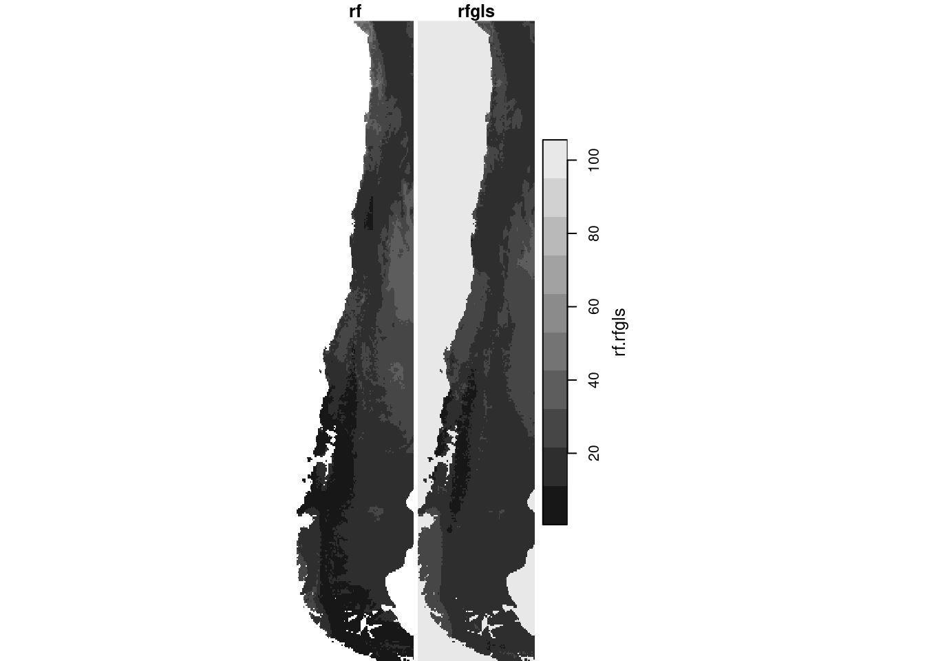
Abhirup Datta has also worked on Neural Networks for Geospatial Data, see this paper (a Python package, no R).
Another package is GPBoost, an R package that allows for combining tree-boosting with Gaussian process and mixed effects models; GPBoost is C++ software and also has a Python interface.
4.6 Exercises
- Carry out an
aoaanalysis using a random forest model fitted using the first 20 distance fields of the last random forest example for NO2 above.- as done in the aoa above, create
yfromno2.sf$NO2, and the selected (first 20) distance fields fromno2.sf - plot the aoa object (distance distribution comparison), the DI field, and the map of the area of applicability
- as done in the aoa above, create
Further reading:
- Hanna Meyer, Edzer Pebesma, 2021. Predicting into unknown space? Estimating the area of applicability of spatial prediction models. Methods in Ecology and Evolution 12 (9), 1620-1633
- Hanna Meyer, Edzer Pebesma, 2022. Machine learning-based global maps of ecological variables and the challenge of assessing them. Nature Communications volume 13, Article number: 2208 (2022)
- J van den Hoogen, N Robmann, D Routh, T Lauber, N van Tiel, O Danylo, TW Crowther, 2021. A geospatial mapping pipeline for ecologists. BioRxiv