## Geostatistical data
### Learning goals
- Get familiar with geostatistical data and spatial interpolation
- Get familiar with concepts of geostatistics: stationarity, variogram, kriging, conditional simulation
- Get an idea what spatiotemporal geostatistics is about
### Reading materials
From [Spatial Data Science: with applications in R](https://r-spatial.org/book/):
- Chapter 12: Spatial Interpolation
- Chapter 13: Multivariate and Spatiotemporal Geostatistics
::: {.callout-tip title="Summary"}
- Intro to `gstat`
- Geostatistical data
- Spatial correlation, variograms, stationarity
- Kriging
- Simulating geostatistical data
- Spatiotemporal geostatistics
:::
## `gstat`
R package `gstat` was written in 2002/3, from a stand-alone C program that was released under the GPL in 1997. It implements "basic" geostatistical functions for modelling spatial dependence (variograms), kriging interpolation and conditional simulation. It can be used for multivariable kriging (cokriging), as well as for spatiotemporal variography and kriging. Recent updates included support for `sf` and `stars` objects.
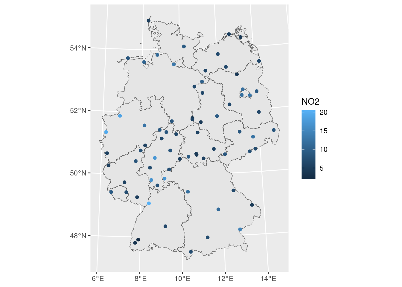
## What are geostatistical data?
Recall from day 1: locations + measured values
- The value of interest is measured at a set of sample locations
- At other location, this value exists but is *missing*
- The interest is in estimating (predicting) this missing value (interpolation)
- The actual sample locations are not of (primary) interest, the signal is in the measured values
```{r}
library(sf)
no2 <- read.csv(system.file("external/no2.csv",
package = "gstat"))
crs <- st_crs("EPSG:32632") # a csv doesn't carry a CRS!
st_as_sf(no2, crs = "OGC:CRS84", coords =
c("station_longitude_deg", "station_latitude_deg")) |>
st_transform(crs) -> no2.sf
library(ggplot2)
# plot(st_geometry(no2.sf))
"https://github.com/edzer/sdsr/raw/main/data/de_nuts1.gpkg" |>
read_sf() |>
st_transform(crs) -> de
ggplot() + geom_sf(data = de) +
geom_sf(data = no2.sf, mapping = aes(col = NO2))
```
## Spatial correlation
### Lagged scatterplots
"by hand", base R:
```{r}
(w = st_is_within_distance(no2.sf, no2.sf, units::set_units(50, km),
retain_unique = TRUE))
d = as.data.frame(w)
x = no2.sf$NO2[d$row.id]
y = no2.sf$NO2[d$col.id]
cor(x, y)
plot(x, y, main = "lagged scatterplot")
abline(0, 1)
```
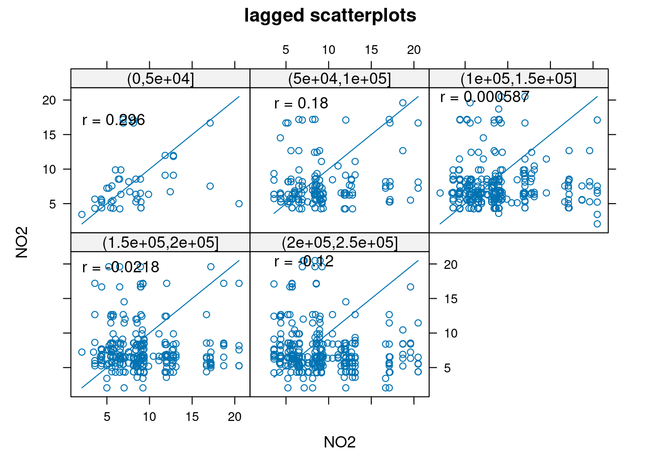
using gstat:
```{r}
library(gstat)
hscat(NO2~1, no2.sf, breaks = c(0,50,100,150,200,250)*1000)
```
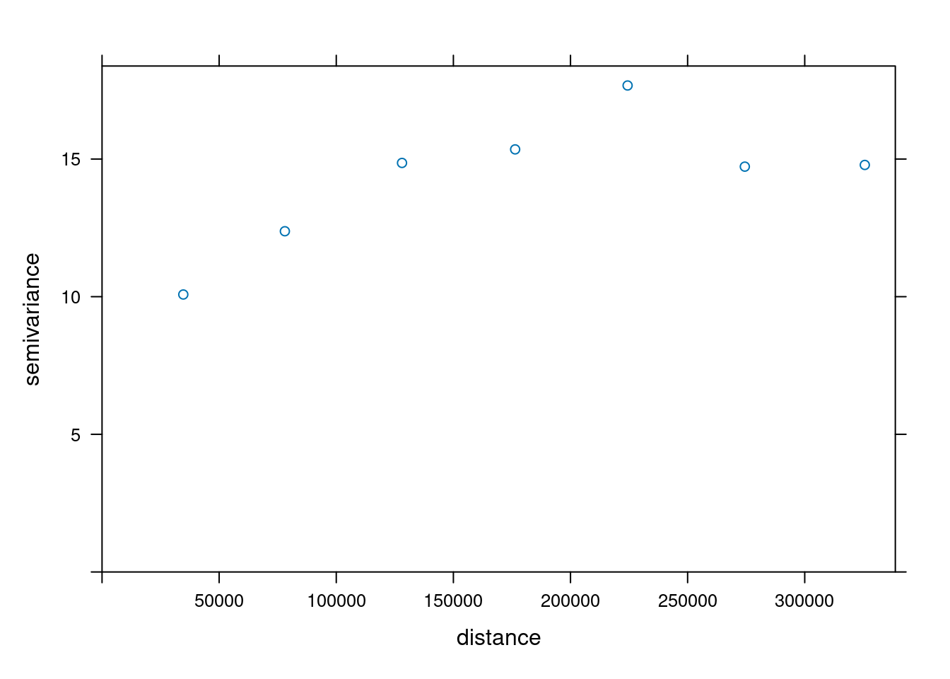
### Variogram
When we assume $Z(s)$ has a constant and unknown mean, the spatial dependence can be described by the variogram, defined as $\gamma(h)
= 0.5 E(Z(s)-Z(s+h))^2$. If the random process $Z(s)$ has a finite variance, then the variogram is related to the covariance function $C(h)$ by $\gamma(h) = C(0)-C(h)$.
The variogram can be estimated from sample data by averaging squared differences: $$\hat{\gamma}(\tilde{h})=\frac{1}{2N_h}\sum_{i=1}^{N_h}(Z(s_i)-Z(s_i+h))^2 \ \
h \in \tilde{h}$$
- divide by $2N_h$:
- if finite, $\gamma(\infty)=\sigma^2=C(0)$
- *semi* variance
- if data are not gridded, group $N_h$ pairs $s_i,s_i+h$ for which $h \in \tilde{h}$, $\tilde{h}=[h_1,h_2]$
- rule-of-thumb: choose about 10-25 distance intervals $\tilde{h}$, from length 0 to about on third of the area size
- plot $\gamma$ against $\tilde{h}$ taken as the average value of all $h \in \tilde{h}$
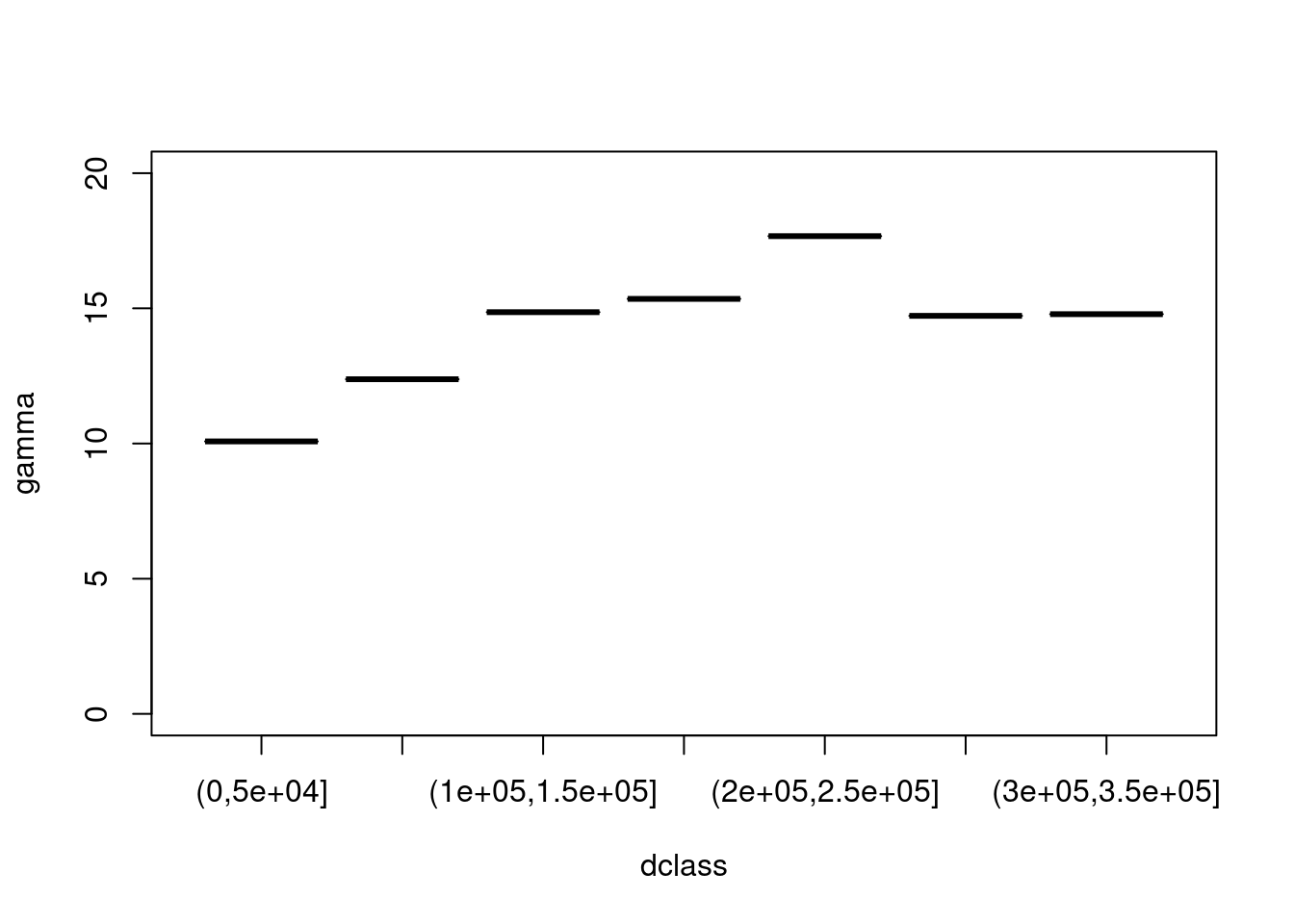
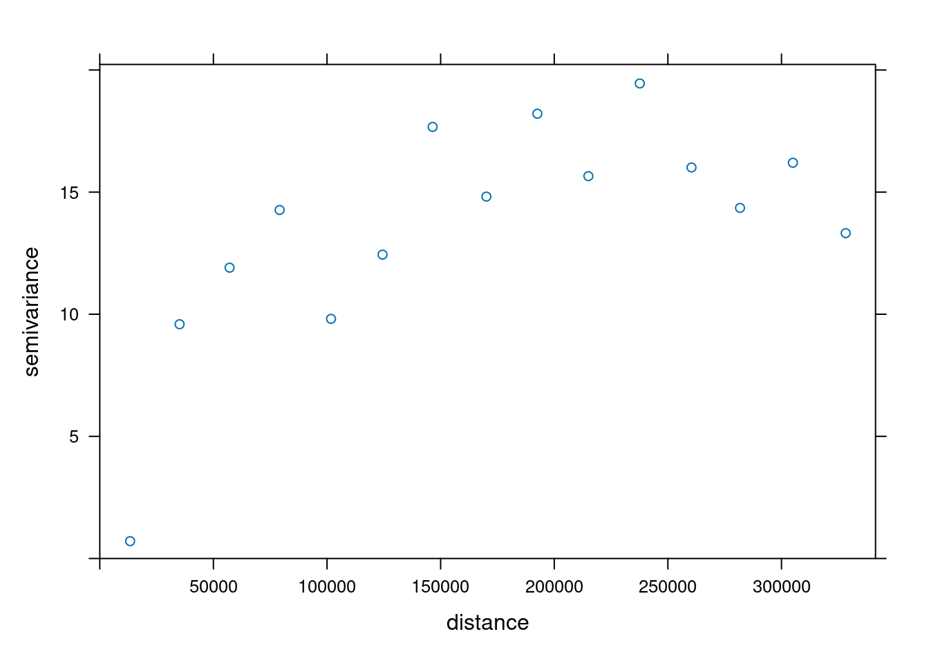
We can compute a variogram "by hand", using base R:
```{r}
z = no2.sf$NO2
z2 = 0.5 * outer(z, z, FUN = "-")^2 # (Z(s)-Z(s+h))^2
d = as.matrix(st_distance(no2.sf))  # h
vcloud = data.frame(dist = as.vector(d), gamma = as.vector(z2))
vcloud = vcloud[vcloud$dist != 0,]
vcloud$dclass = cut(vcloud$dist, c(0, 50, 100, 150, 200, 250, 300, 350) * 1000)
v = aggregate(gamma~dclass, vcloud, mean)
plot(gamma ~ dclass, v, ylim = c(0, 20))
```
using gstat:
```{r}
vv = variogram(NO2~1, no2.sf, width = 50000, cutoff = 350000)
vv$gamma - v$gamma
plot(vv)
```
## Exercises
1. Compute the variogram cloud of NO2 using `variogram()` and argument `cloud = TRUE`. (a) How does the resulting object differ from the "regular" variogram (use the `head` command on both objects); (b) what do the "left" and "right" fields refer to? (c) when we plot the resulting variogram cloud object, does it still indicate spatial correlation?
2. Compute the variogram of NO2 as above, and change the arguments `cutoff` and `width` into very large or small values. What do they do?
3. Fit a spherical model to the sample variogram of NO2, using `fit.variogram()` (follow the example below, replace "Exp" with "Sph")
4. Fit a Matern model ("Mat") to the sample variogram using different values for kappa (e.g., 0.3 and 4), and plot the resulting models with the sample variogram.
5. Which model do you like the best? Can the SSErr attribute of the fitted model be used to compare the models? How else can variogram model fits be compared?
## Interpolation
For interpolation, we first need a target grid (point patterns have an observation window, geostatistical data do not!)
A simple interpolator (that is hard to beat) is the inverse distance interpolator, $$\hat{Z}(s_0) = \sum_{j=1}^n \lambda_j Z(s_i)$$ with $\lambda_j$ proportional to $||s_i - s_0||^{-p}$ and normalized to sum to one (weighted mean), and $p$ tunable but defaulting to 2.
Using the data range:
```{r}
library(stars)
g1 = st_as_stars(st_bbox(no2.sf))
library(gstat)
idw(NO2~1, no2.sf, g1) |> plot(reset = FALSE)
plot(st_geometry(no2.sf), add = TRUE, col = 'yellow')
plot(st_cast(st_geometry(de), "MULTILINESTRING"), add = TRUE, col = 'red')
```
Better to use the outer polygon:
```{r}
g2 = st_as_stars(st_bbox(de))
idw(NO2~1, no2.sf, g2) |> plot(reset = FALSE)
plot(st_geometry(no2.sf), add = TRUE, col = 'yellow')
plot(st_cast(st_geometry(de), "MULTILINESTRING"), add = TRUE, col = 'red')
```
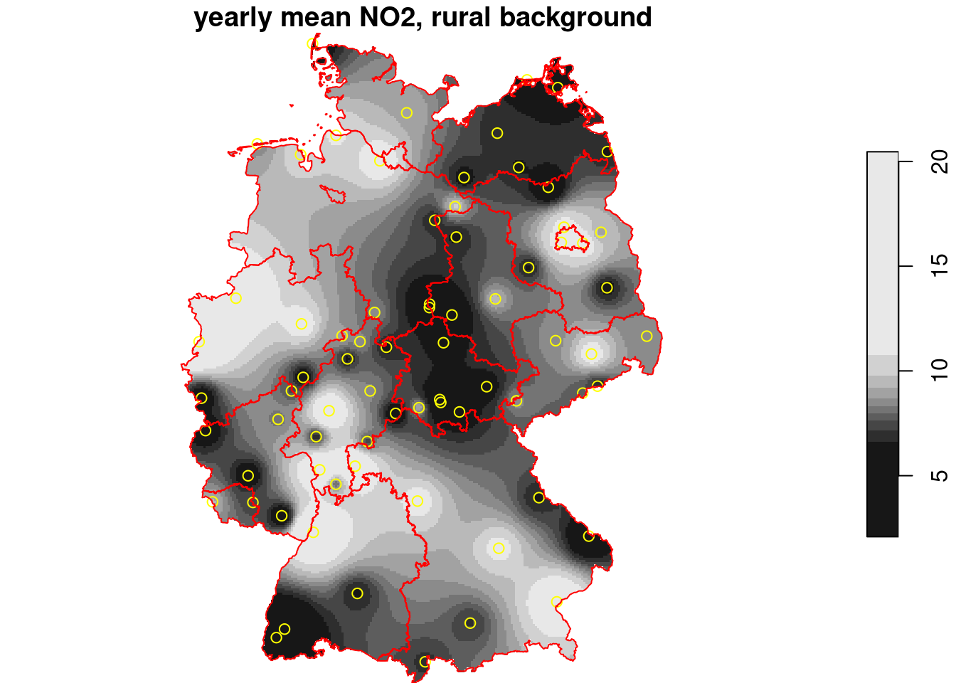
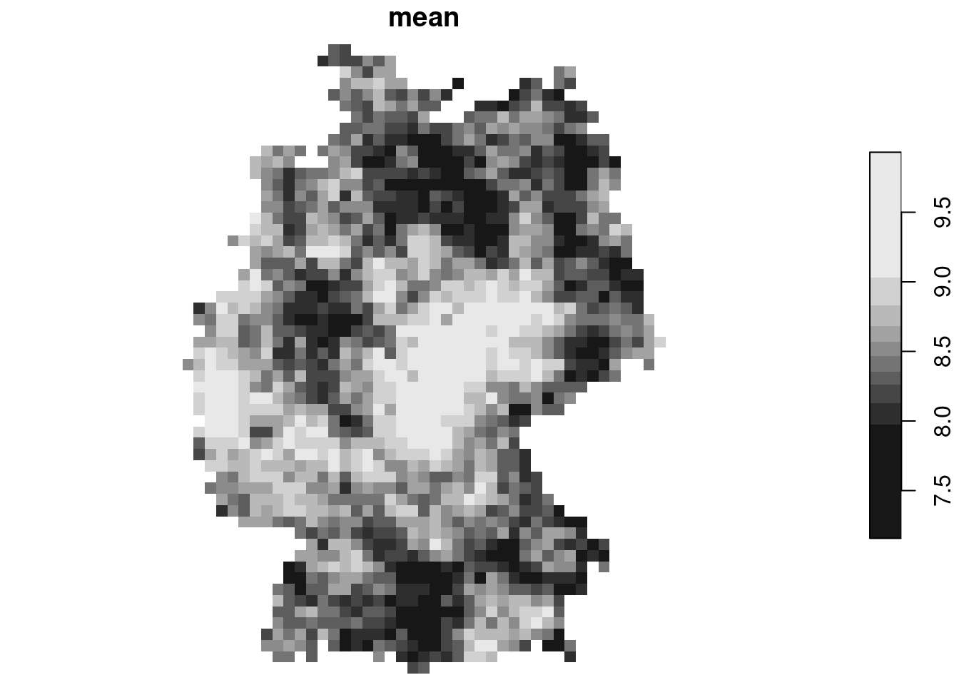
And crop to (mask out outside) the area of interest:
```{r}
g3 = st_crop(g2, de)
i = idw(NO2~1, no2.sf, g3)
plot(i, reset = FALSE, main = "yearly mean NO2, rural background")
plot(st_geometry(no2.sf), add = TRUE, col = 'yellow')
plot(st_cast(st_geometry(de), "MULTILINESTRING"), add = TRUE, col = 'red')
```
Geostatistical approaches compute weights based on covariances between observations $Z(s_i)$, and between observations and the value at the interpolation location $Z(s_0)$. These covariances are obtained from a model fitted to the sample variogram.
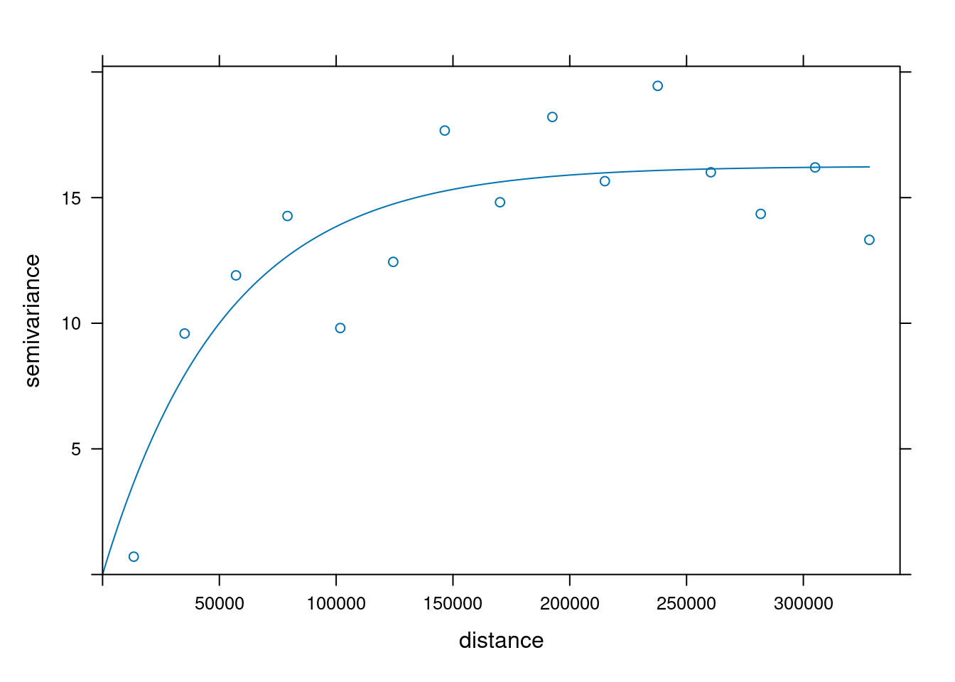
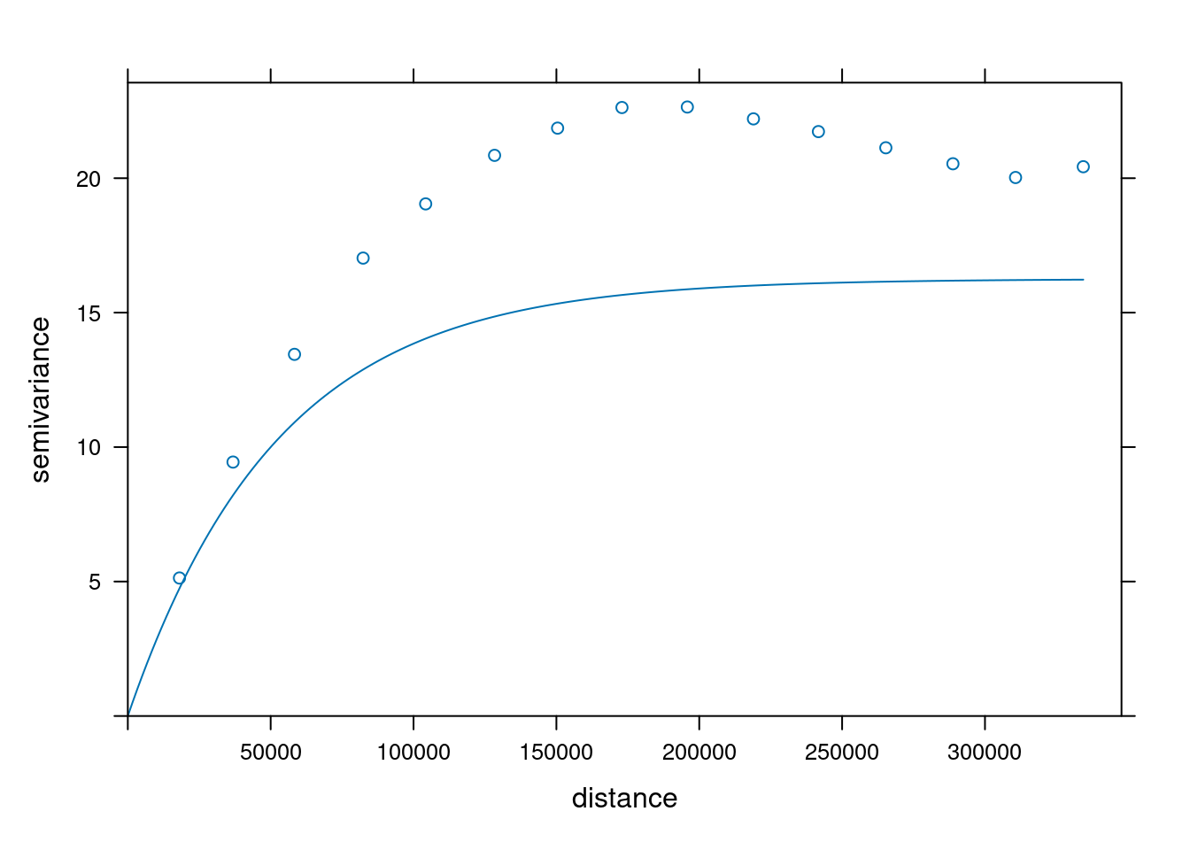
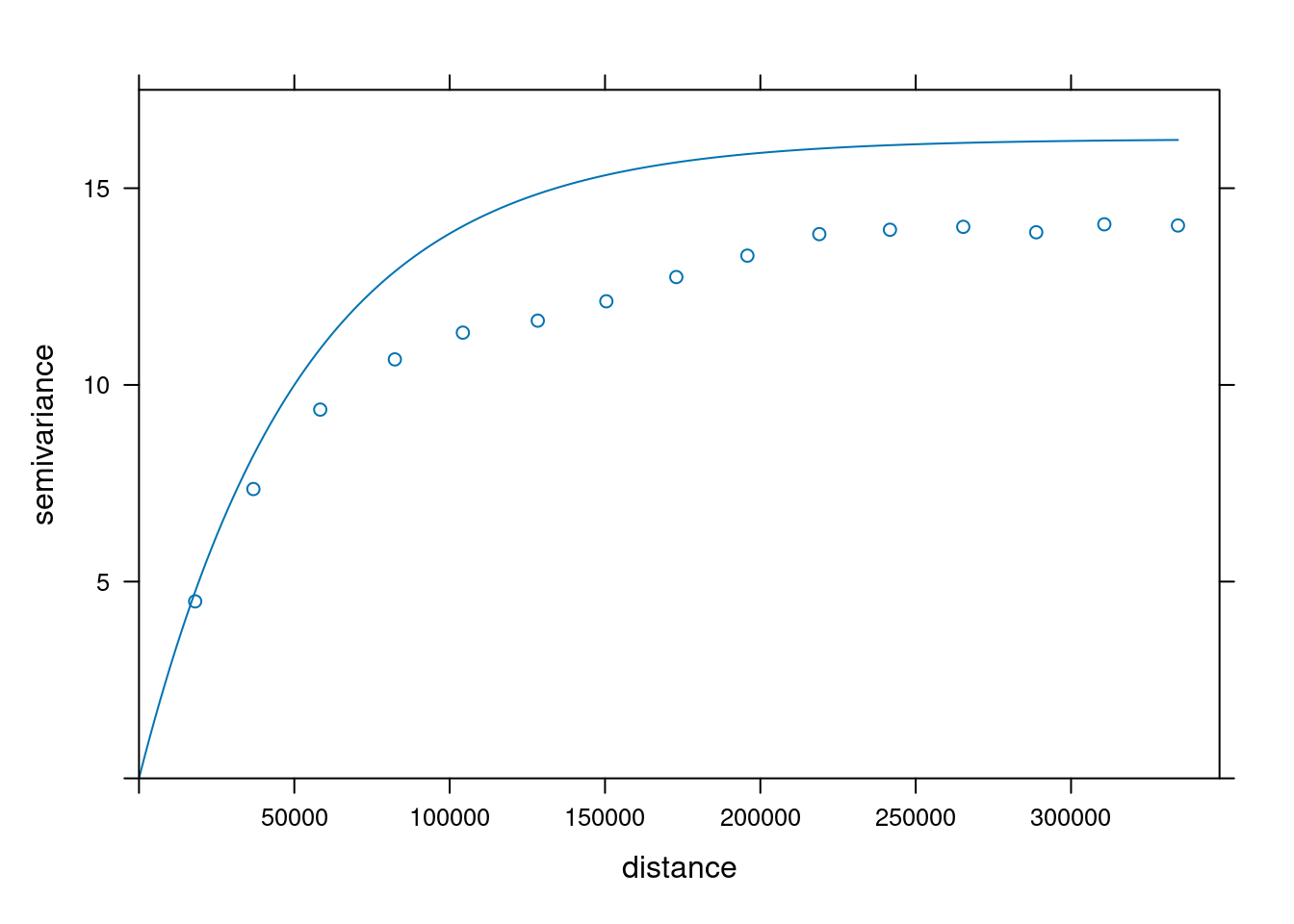
## Fit a variogram model
```{r}
# The sample variogram:
v = variogram(NO2~1, no2.sf)
plot(v)
```
fit a model, e.g. an exponential model:
```{r}
v.fit = fit.variogram(v, vgm(1, "Exp", 50000))
plot(v, v.fit)
```
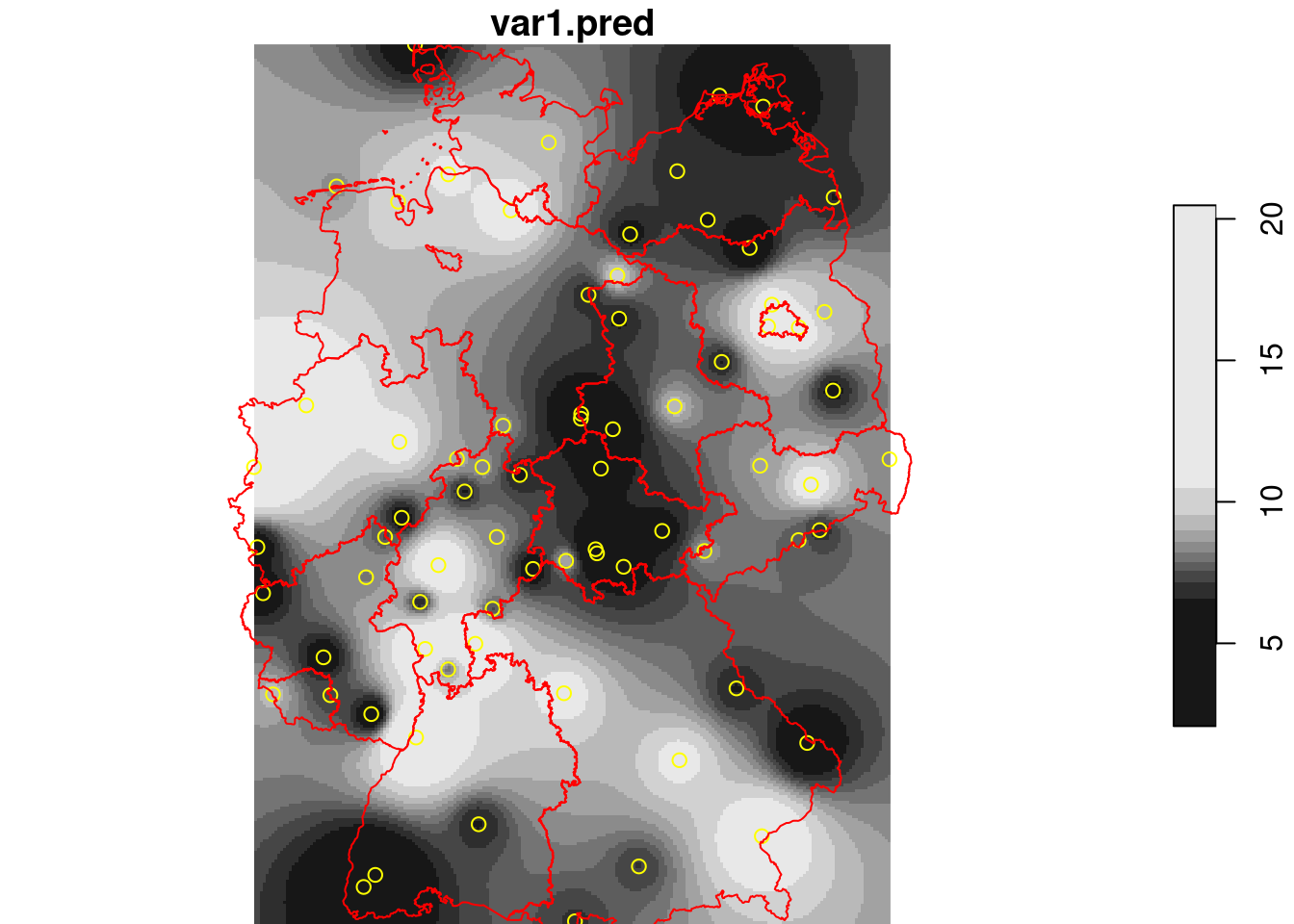
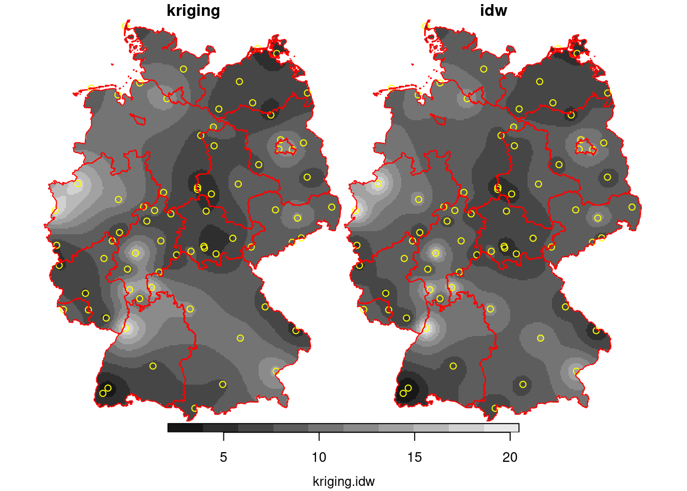
## BLUP/Kriging
Given this model, we can interpolate using the *best unbiased linear predictor* (BLUP), also called kriging predictor. Under the model $Z(s)=m+e(s)$ it estimates $m$ using generalized least squares, and predicts $e(s)$ using a weighted mean, where weights are chosen such that $Var(Z(s_0)-\hat{Z}(s_0))$ is minimized.
```{r}
k = krige(NO2~1, no2.sf, g3, v.fit)
k$idw = i$var1.pred
k$kriging = k$var1.pred
hook = function() {
plot(st_geometry(no2.sf), add = TRUE, col = 'yellow')
plot(st_cast(st_geometry(de), "MULTILINESTRING"), add = TRUE, col = 'red')
}
plot(merge(k[c("kriging", "idw")]), hook = hook, breaks = "equal")
```
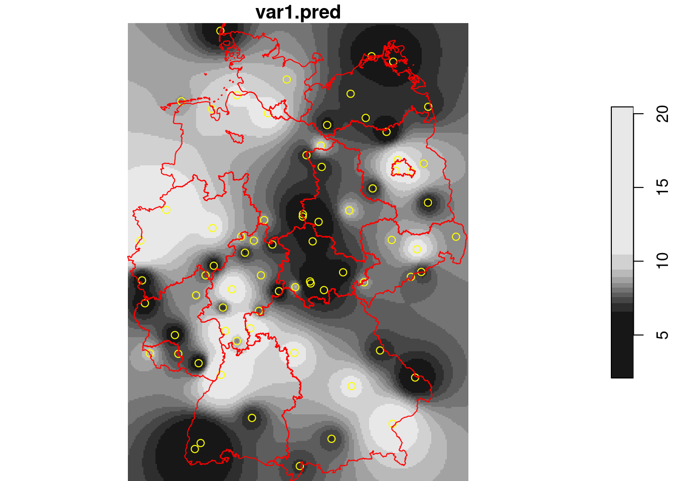
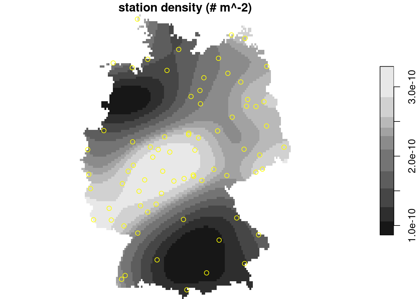
::: callout-important
## Density or interpolation?
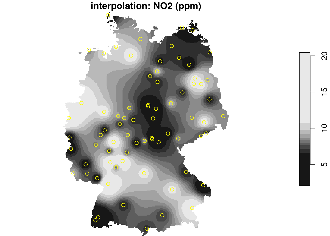
Both density maps shown in the Point Pattern section and interpolated maps shown in this section look very similar:
- raster maps with continuous values
- smooth spatial patterns
The differences could not be larger!
- point density estimates estimate the number of points per unit area; the values are (normalized) *counts*
- interpolated maps estimate an unmeasured continuous variable; the values are weighted averages of an *attribute*
:::
To illustrate the difference between density and interpolated values:
```{r echo=FALSE}
#| code-fold: true
#| out.width: '100%'
library(spatstat)
p = as.ppp(st_geometry(no2.sf), W = as.owin(st_union(st_geometry(de))))
density(p) |> st_as_stars() |> plot(main = "station density (# m^-2)", reset = FALSE)
plot(st_geometry(no2.sf), add = TRUE, col = 'yellow')
```
```{r echo=FALSE}
#| code-fold: true
#| out.width: '100%'
plot(i, main = "interpolation: NO2 (ppm)", reset = FALSE)
plot(st_geometry(no2.sf), add = TRUE, col = 'yellow')
```
## Kriging with a non-constant mean
Under the model $Z(s) = X(s)\beta + e(s)$, $\beta$ is estimated using generalized least squares, and the variogram of regression residuals is needed; see Ch 12.
## Conditional simulation
### Simulating spatially correlated data
Using a coarse grid, with base R:
```{r}
set.seed(13579)
g2c = st_as_stars(st_bbox(de), dx = 15000)
g3c = st_crop(g2c, de)
p = st_as_sf(g3c, as_points = TRUE)
d = st_distance(p)
Sigma = variogramLine(v.fit, covariance = TRUE, dist_vector = d)
n = 100
ch = chol(Sigma)
sim = matrix(rnorm(n * nrow(ch)), nrow = n) %*% ch + mean(no2.sf$NO2)
for (i in seq_len(n)) {
    m = g3c[[1]]
    m[!is.na(m)] = sim[i,]
    g3c[[ paste0("sim", i) ]] = m
}
plot(merge(g3c[2:11]), breaks = "equal")
```
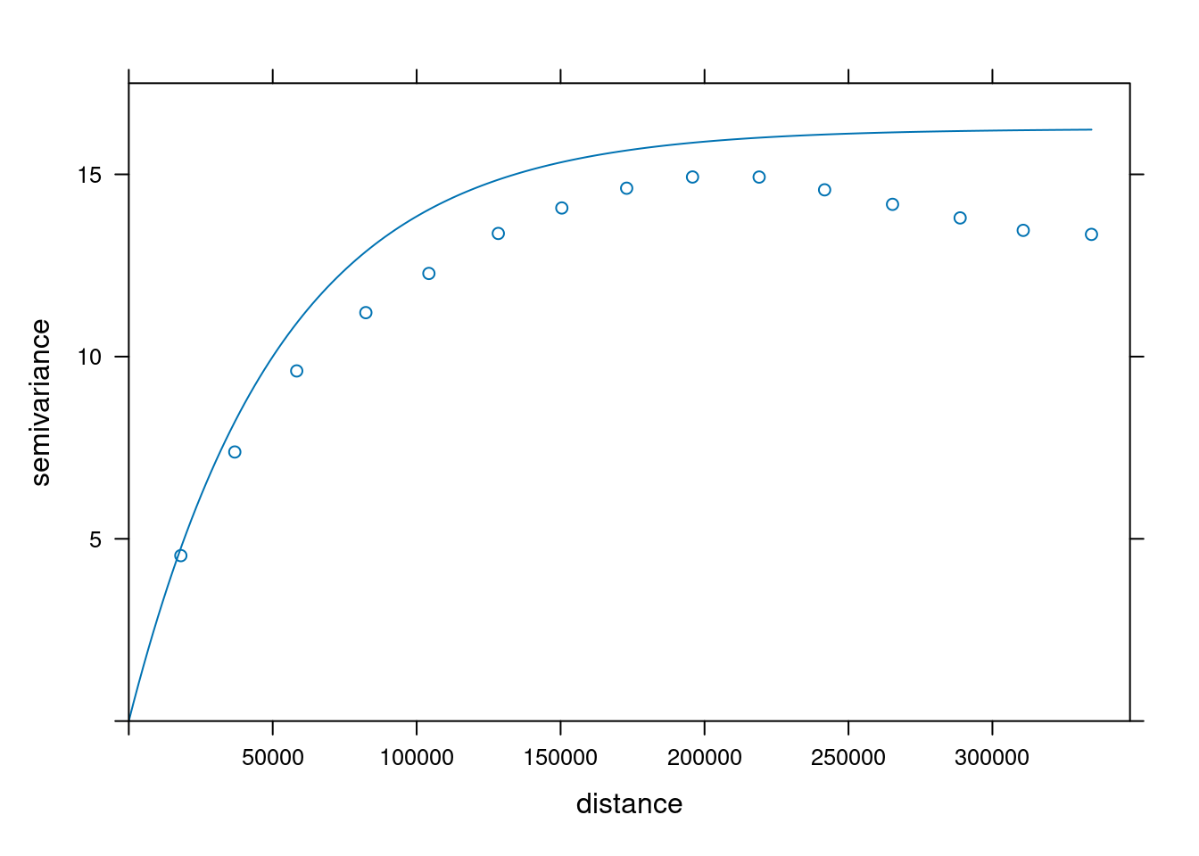
As a check, we could compute the variogram of some of the realisations:
```{r}
g3c["sim4"] |>
  st_as_sf() |>
  variogram(sim4~1, data = _) |>
  plot(model = v.fit)
g3c["sim5"] |>
  st_as_sf() |>
  variogram(sim5~1, data = _) |>
  plot(model = v.fit, ylim = c(0,17.5))
g3c["sim6"] |>
  st_as_sf() |>
  variogram(sim6~1, data = _) |>
  plot(model = v.fit, ylim = c(0,17.5))
```
The mean of these simulations is constant, not related to measured values:
```{r}
st_apply(merge(g3c[-1]), c("x", "y"), mean) |> plot()
mean(no2.sf$NO2)
```
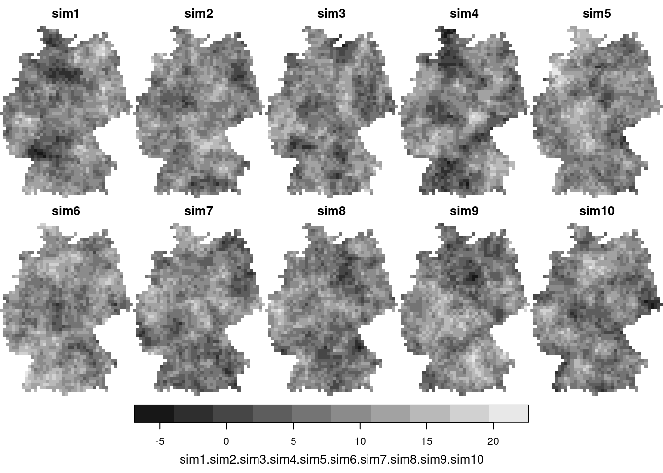
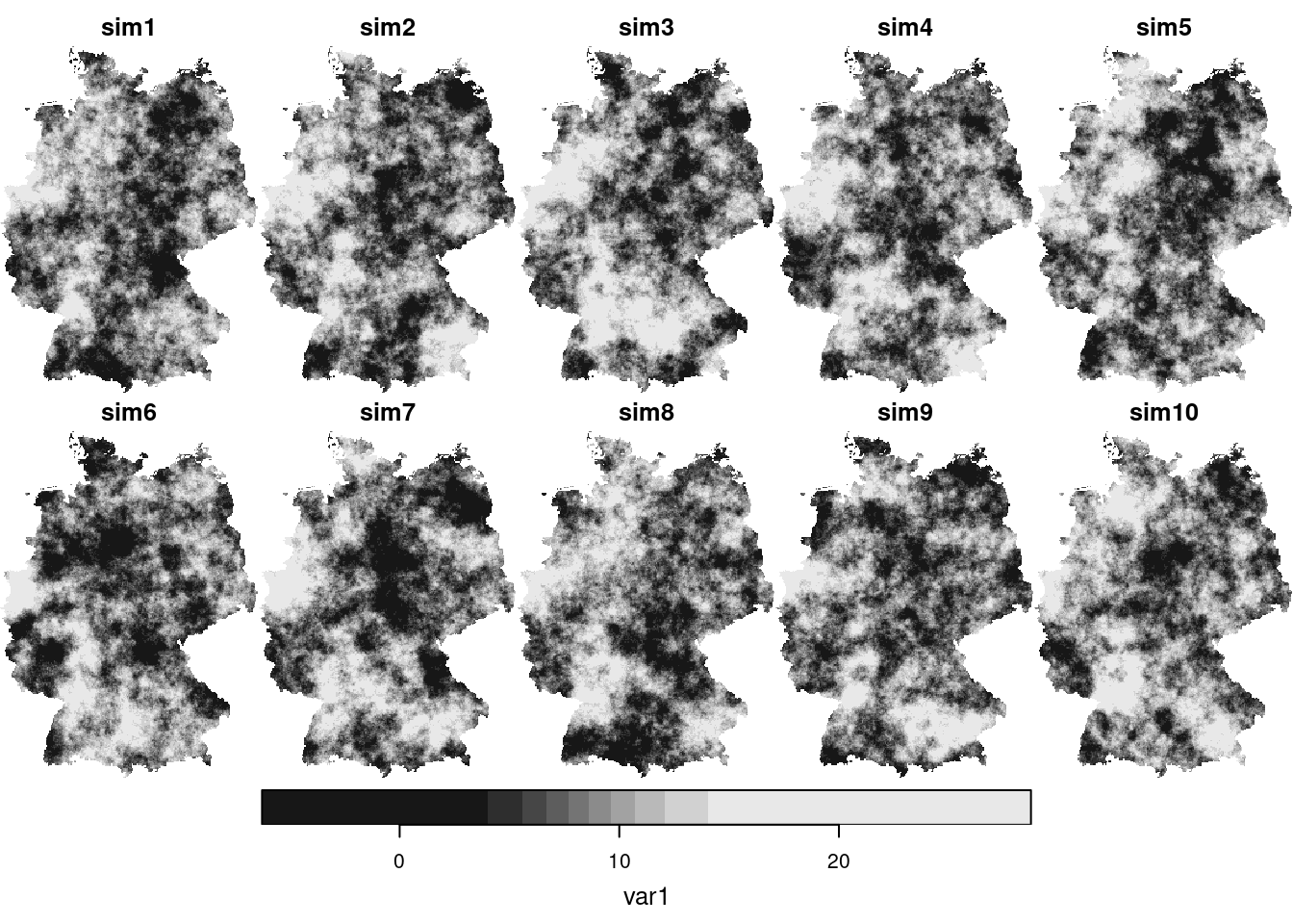
Conditioning simulations on measured values can be done with `gstat`, using *conditional simulation*
```{r}
cs = krige(NO2~1, no2.sf, g3, v.fit, nsim = 50, nmax = 30)
plot(cs[,,,1:10])
```
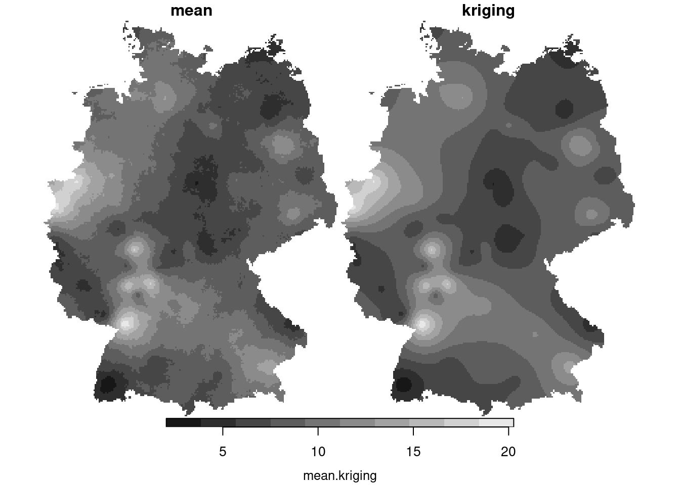
We see that these simulations are much more alike; also their mean and variance resemble that of the kriging mean and variance:
```{r}
csm = st_apply(cs, c("x", "y"), mean)
csm$kriging = krige(NO2~1, no2.sf, g3, v.fit)[1]
plot(merge(csm), breaks = "equal")
csv = st_apply(cs, c("x", "y"), var)
csv$kr_var = krige(NO2~1, no2.sf, g3, v.fit)[2]
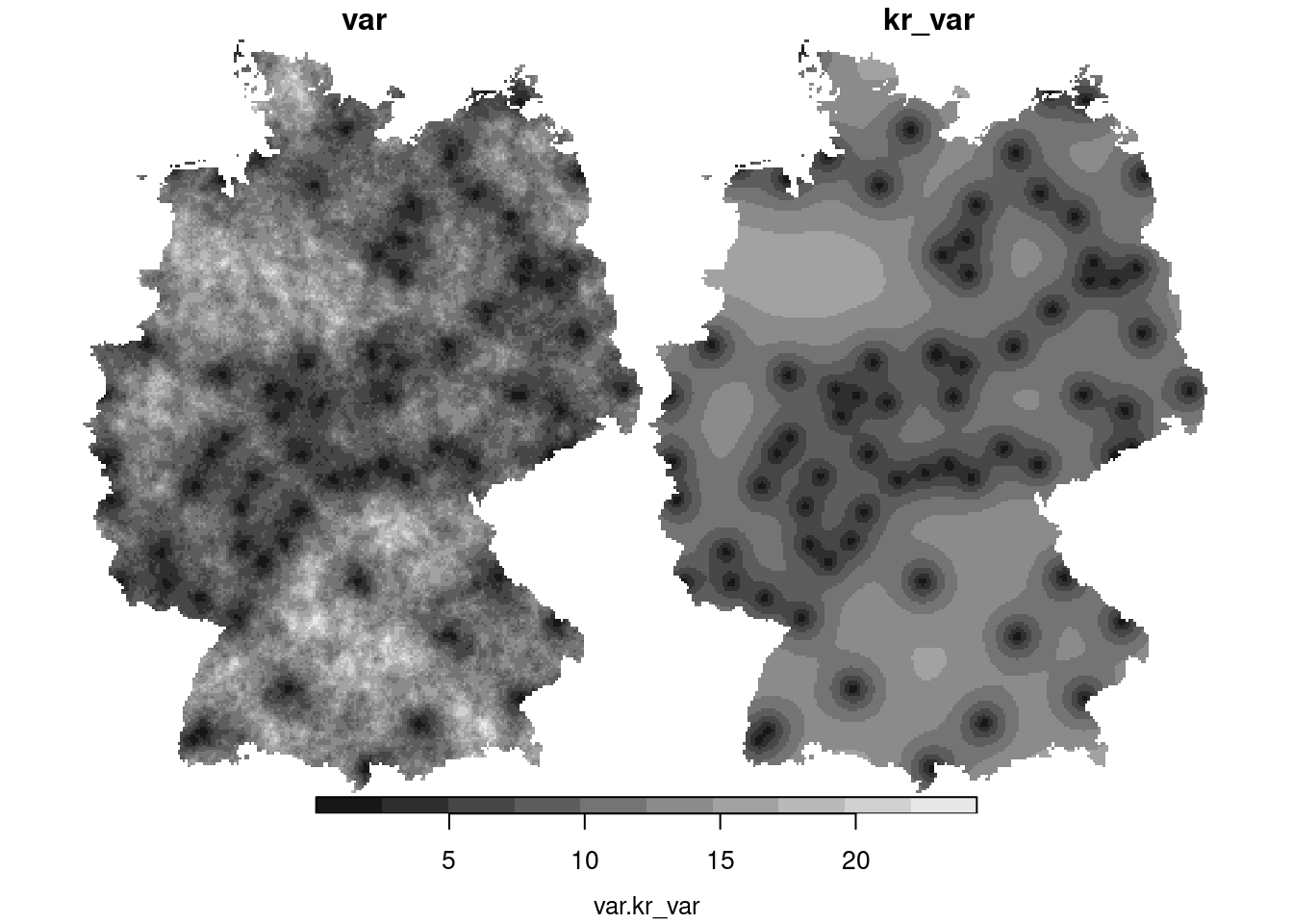
plot(merge(csv), breaks = "equal")
```
## Exercises
1. What causes the differences between the mean and the variance of
the simulations (left) and the mean and variance obtained by kriging
(right)?
2. When comparing (above) the sample variogram of simulated fields
with the variogram model used to simulate them, where do you
see differences? Can you explain why these are not identical, or
hypothesize under which circumstances these would become (more)
identical?
3. Under which practical data analysis problem would conditional
simulations be more useful than the kriging prediction + kriging
variance maps?
## Further reading
- Pebesma, E.J., 2004. Multivariable geostatistics in S: the gstat package. Computers & Geosciences, 30: [683-691](https://doi.org/10.1016/j.cageo.2004.03.012).
- Benedikt Gräler, Edzer Pebesma and Gerard Heuvelink, 2016. Spatio-Temporal Interpolation using gstat. The R Journal 8(1), [204-218](https://journal.r-project.org/archive/2016/RJ-2016-014/index.html)