5  Simple approaches

\[ \newcommand{\Cor}{{\rm Corr}} \]

5.1 Taking a step back

Why do we need models?

  • to understand relations or processes
  • to assess (predict, forcast, map) something we do or did not measure and cannot see
  • to assess the consequence of decisions (scenarios) where we cannot measure

A sample dataset

The meuse dataset is loaded from package sp:

library(sf)
data(meuse.riv, package = "sp")
data(meuse, package = "sp")
meuse.sf = st_as_sf(meuse, coords = c("x", "y"))
meuse.sr = st_sfc(st_polygon(list(meuse.riv)))
br = c(0, 100,200,400,700,1200,2000)
plot(meuse.sf["zinc"], pch = 16,
    breaks = br, at = br, key.pos = 4,
    main = "zinc, ppm", reset = FALSE)
plot(meuse.sr, col = "lightblue", add = TRUE)

Thiessen “polygons”, 1-NN


library(gstat)
data(meuse.grid, package = "sp") # data.frame
library(stars)
meuse.grid = st_as_stars(meuse.grid) # makes it a raster
meuse.grid
# stars object with 2 dimensions and 5 attributes
# attribute(s):
#     part.a         part.b          dist        soil      
#  Min.   :0      Min.   :0      Min.   :0      1   :1665  
#  1st Qu.:0      1st Qu.:0      1st Qu.:0      2   :1084  
#  Median :0      Median :1      Median :0      3   : 354  
#  Mean   :0      Mean   :1      Mean   :0      NA's:5009  
#  3rd Qu.:1      3rd Qu.:1      3rd Qu.:0                 
#  Max.   :1      Max.   :1      Max.   :1                 
#  NA's   :5009   NA's   :5009   NA's   :5009              
#   ffreq     
#  1   : 779  
#  2   :1335  
#  3   : 989  
#  NA's:5009  
#             
#             
#             
# dimension(s):
#   from  to offset delta x/y
# x    1  78 178440    40 [x]
# y    1 104 333760   -40 [y]

meuse.th = idw(zinc~1, meuse.sf, meuse.grid, nmax = 1)
# [inverse distance weighted interpolation]

plot(meuse.th[1], nbreaks = 29, col = sf.colors(28),
    main = "Zinc, 1-nearest neighbour", reset = FALSE)
plot(st_geometry(meuse.sf), col = 3, cex=.5, add = TRUE)

Zinc concentration vs. distance to river

plot(log(zinc)~sqrt(dist), meuse.sf)
abline(lm(log(zinc) ~ sqrt(dist), meuse.sf))

Zinc conc. vs. distance to river: map of linear trend

meuse.grid$sqrtdist = sqrt(meuse.grid$dist)
plot(meuse.grid["sqrtdist"], col = sf.colors(), breaks = "equal")

Inverse distance weighted interpolation

Uses a weighted average: \[\hat{Z}(s_0) = \sum_{i=1}^n \lambda_i Z(s_i)\] with \(s_0 = \{x_0, y_0\}\), or \(s_0 = \{x_0, y_0, \mbox{depth}_0\}\) weights inverse proportional to power \(p\) of distance: \[\lambda_i = \frac{|s_i-s_0|^{-p}}{\sum_{i=1}^n |s_i-s_0|^{-p}}\]

  • power \(p\): tuning parameter
  • if for some \(i\), \(|s_i-s_0| = 0\), then \(\lambda_i = 1\) and other weights become zero
  • \(\Rightarrow\) exact interpolator

Effect of power \(p\)

set.seed(13531)
pts = data.frame(x = 1:10, y = rep(0,10), z = rnorm(10)*3 + 6)
pts.sf = st_as_sf(pts, coords = c("x", "y"))
xpts = 0:1100 / 100
grd = data.frame(x = xpts, y = rep(0, length(xpts)))
grd = st_as_sf(grd, coords = c("x", "y"))
plot(z ~ x, as.data.frame(pts), xlab ='location', ylab = 'attribute value')
lines(xpts, idw(z~1, pts.sf, grd, idp = 2)$var1.pred)
# [inverse distance weighted interpolation]
lines(xpts, idw(z~1, pts.sf, grd, idp = 5)$var1.pred, col = 'darkgreen')
# [inverse distance weighted interpolation]
lines(xpts, idw(z~1, pts.sf, grd, idp = .5)$var1.pred, col = 'red')
# [inverse distance weighted interpolation]
legend("bottomright", c("2", ".5", "5"), lty = 1, 
    col=c("black", "red", "darkgreen"), title = "invese distance power")

Time series versus spatial data

Differences:

  • spatial data live in 2 (or 3) dimensions
  • there’s no past and future
  • there’s no simple conditional independence (AR)

Correspondences

  • nearby observations are more alike (auto-correlation)
  • we can form moving averages
  • coordinate reference systems are a bit like time zones and DST

What information do we have?

  • We have measurements \(Z(x)\), with \(x\) two-dimensional (location on the map)
  • we have \(x\) and \(y\)
  • we may have land use data
  • we may have soil type or geological data
  • we may have remote sensing imagery
  • we may have all kinds of relevant information, related to processes that cause (or result from) \(Z(x)\)
  • we have google maps and other tiled web map sources

We don’t want to ignore anything important

Regression or correlation?

(Correlation between two different variables, no auto-correlation:)

n = 500
x = rnorm(n)
y = rnorm(n)
R = matrix(c(1,0,0,1),2,2)
R
#      [,1] [,2]
# [1,]    1    0
# [2,]    0    1
plot(cbind(x,y) %*% chol(R))
title("zero correlation")

R[2,1] = R[1,2] = 0.5
plot(cbind(x,y) %*% chol(R))
title("correlation 0.5")

R[2,1] = R[1,2] = 0.9
plot(cbind(x,y) %*% chol(R))
title("correlation 0.9")

R[2,1] = R[1,2] = 0.98
plot(cbind(x,y) %*% chol(R))
title("correlation 0.98")

Correlation vs. regression:

Correspondences:

  • both are in the “classic statistics” book, and may involve hypothesis testing
  • both deal with two continuous variables
  • both look at (first order) linear relations
  • when correlation is significant, the regression slope is significant

Differences:

  • Regression distinguishes \(y\) from \(x\): \(y\) depends on \(x\), not reverse;
  • the line \(y=ax+b\) is not equal to the line \(x = cy + d\)
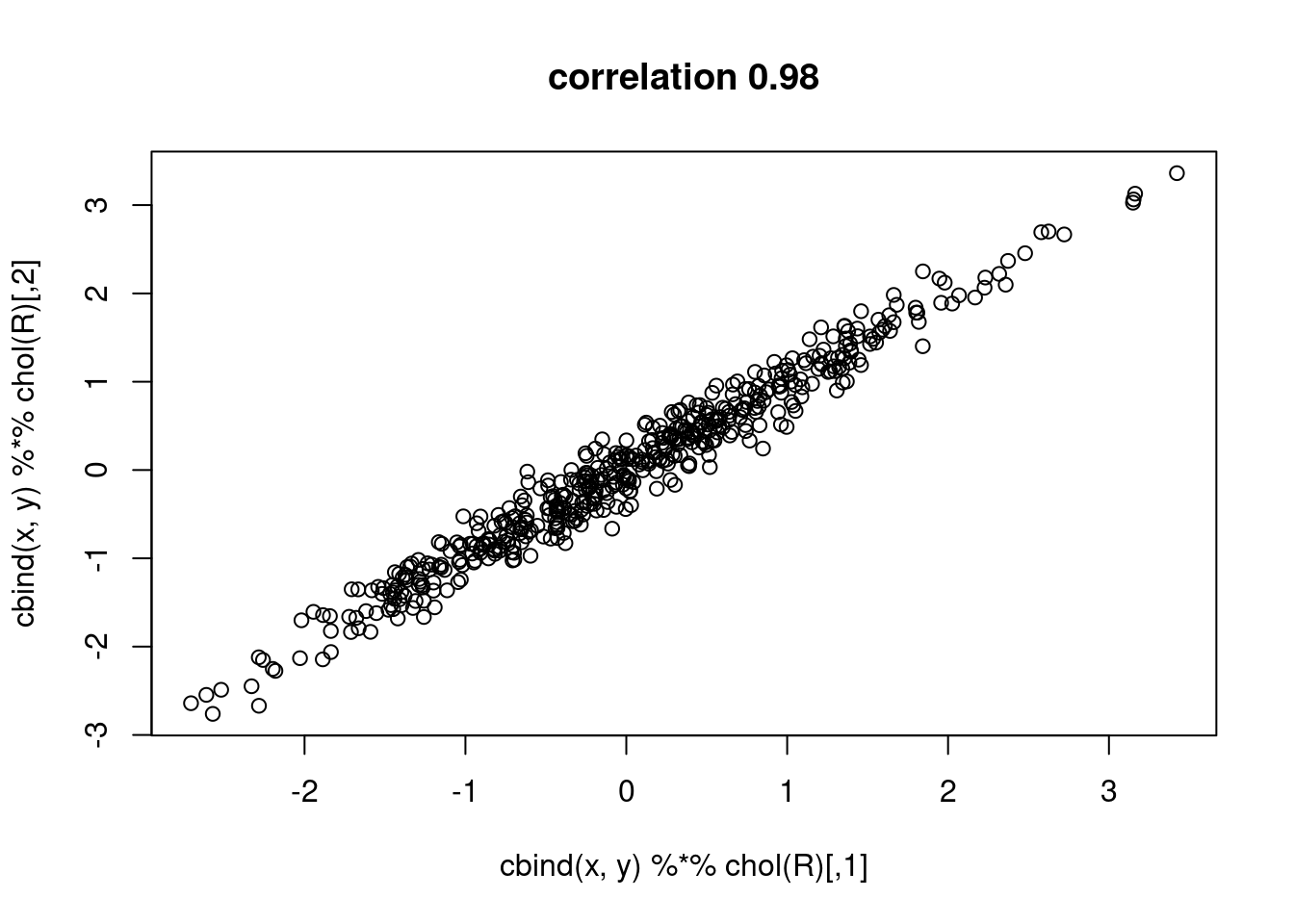
  • Correlation is symmetric: \(\Cor(x,y)=\Cor(y,x)\)
  • Correlation coefficient is unitless and within \([-1,1]\), regression coeficients have data units
  • Regression is concerned with prediction of \(y\) from \(x\).

The power of regression models for spatial prediction

… is hard to overestimate. Regression and correlation are the fork and knife of statistics.

  • linear models have endless application: polynomials, interactions, nested effects, ANOVA/ANCOVA models, hypothesis testing, lack of fit testing, …
  • predictors can be transformed non-linearly
  • linear models can be generalized: logistic regression, Poisson regression, …, to cope with discrete data (0/1 data, counts, log-normal)
  • many derived techniques solve one particular issue in regression, e.g.:
    • ridge regression solves collinearity (extreme correlation among predictors)
    • stepwise regression automatically selects “best” models among many candidates
    • classification and regression trees

Why is regression difficult in spatial problems?

Regression models assume independent observations. Spatial data are always to some degree spatially correlated.

This does not mean we should discard regression, but rather think about

  • to which extent is an outcome dependent on independence?
  • to which extent is regression robust agains a violated assumption of independent observations?
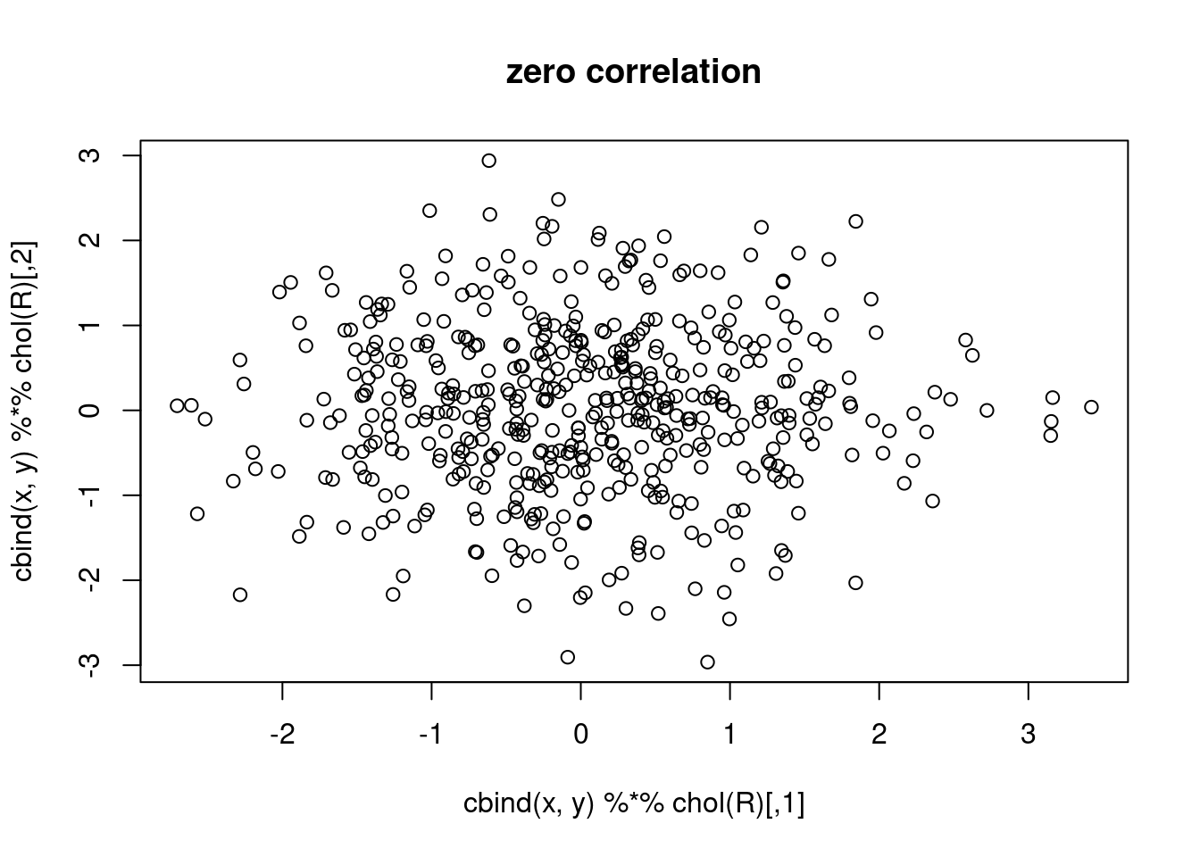
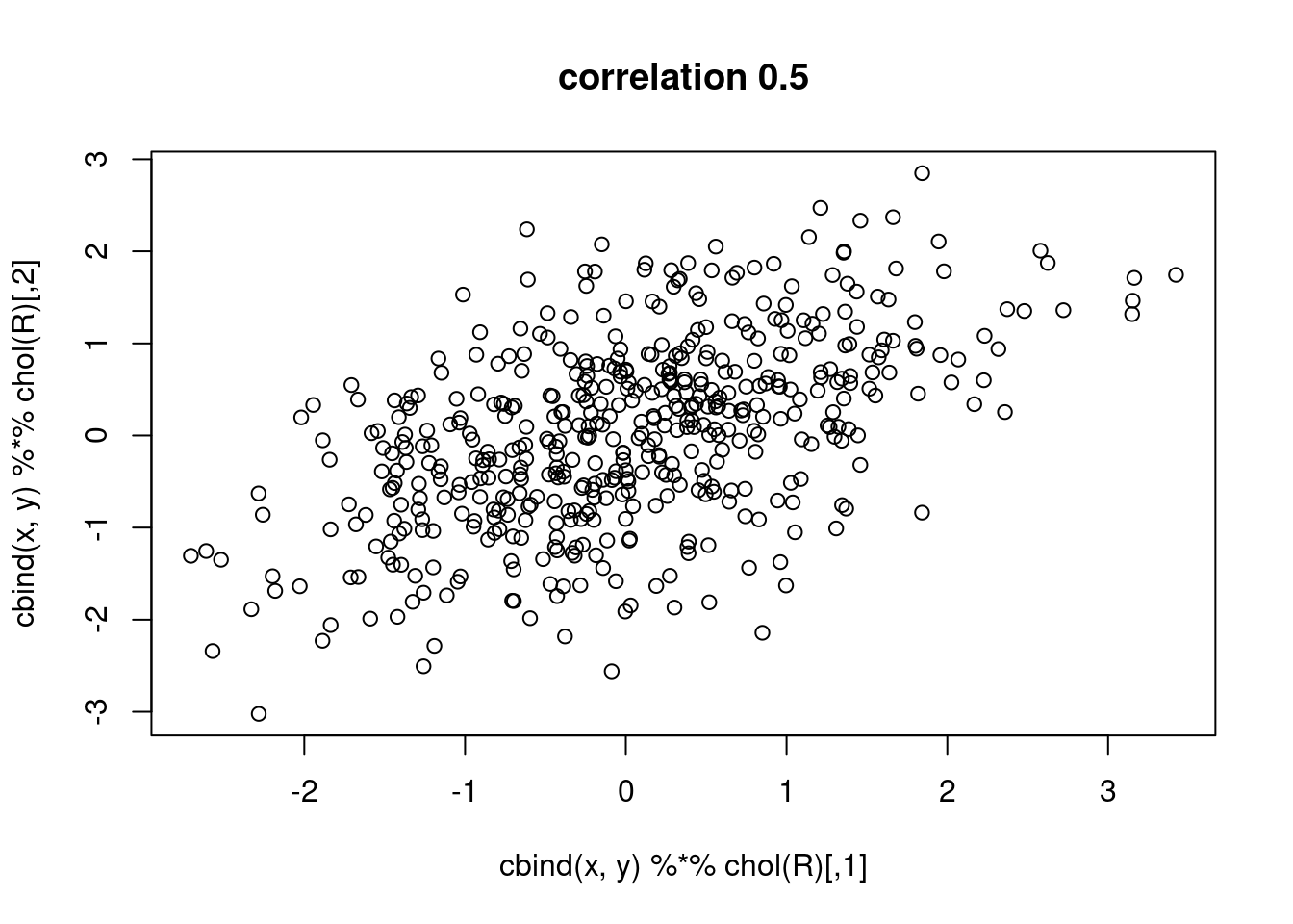
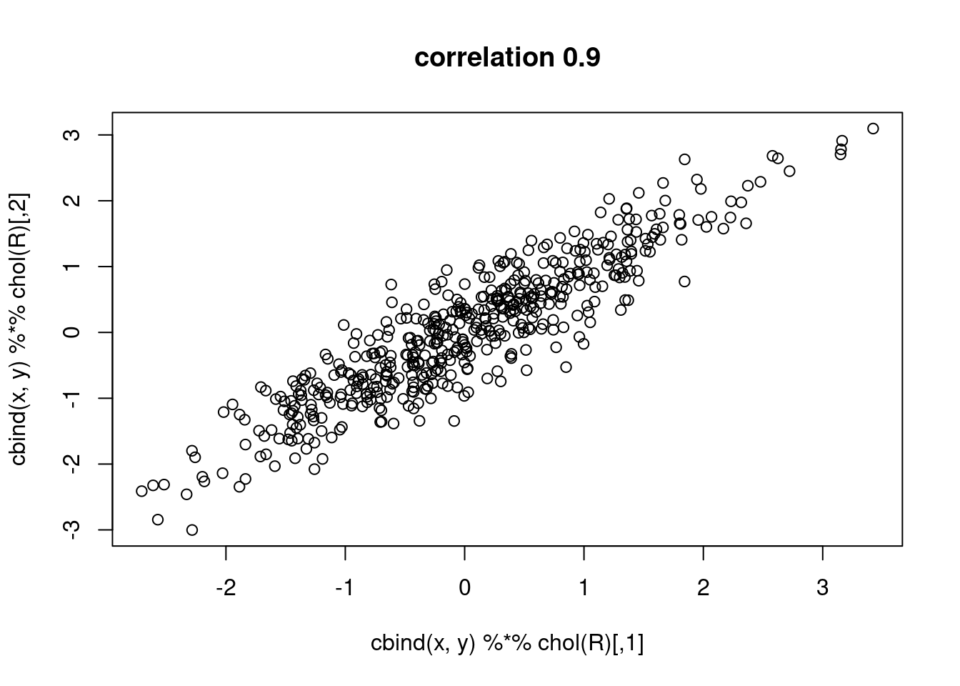
  • to which extent is the assumption violated? (how strong is the correlation)

What is spatial correlation?

Waldo Tobler’s first “law” in geography: “Everything is related to everything else, but near things are more related than distant things.” (Tobler 1970)

Setting aside whether Tobler was the first to acknowledge this, and also whether the expression can be called a “law”, we wonder how being related can be expressed?