library(sf)
data(meuse, package = "sp")
meuse = st_as_sf(meuse, coords = c("x", "y"))
library(gstat)
v = variogram(log(zinc) ~ 1, meuse)
v.fit = fit.variogram(v, vgm(1, "Sph", 900, 1))
plot(v, v.fit)
\[ \newcommand{\E}{{\rm E}} % E expectation operator \newcommand{\Var}{{\rm Var}} % Var variance operator \newcommand{\Cov}{{\rm Cov}} % Cov covariance operator \newcommand{\Cor}{{\rm Corr}} \]
Suppose the mean is constant, but not known. This is the most simple realistic scenario. We can estimate it from the data, taking into account their covariance (i.e., using weighted averaging):
\[\hat{m} = ({\bf 1}'V^{-1}{\bf 1})^{-1} {\bf 1}'V^{-1}Z\] with \({\bf 1}\) a conforming vector with ones, and substitute this mean in the SK prediction equations: BLUP/Ordinary kriging: \[\hat{Z}(s_0) = \hat{m} + v'V^{-1} (Z-\hat{m})\] \[\sigma^2(s_0) = \sigma^2_0 - v'V^{-1}v + Q\] with \(Q = (1 - {\bf 1}'V^{-1}v)'({\bf 1}'V^{-1}{\bf 1})^{-1}(1 - {\bf 1}'V^{-1}v)\)
Given prediction location \(s_0\), and data locations \(s_1\) and \(s_2\), we need: \(\Var(Z(s_0))\), \(\Var(Z(s_1))\), \(\Var(Z(s_2))\), \(\Cov(Z(s_0),Z(s_1))\), \(\Cov(Z(s_0),Z(s_2))\), \(\Cov(Z(s_1),Z(s_2))\).
How to get these covariances?
Solution: assume stationarity.
Stationarity of the
Second order stationarity: \(\Cov(Z(s),Z(s+h)) = C(h)\)
which implies: \(\Cov(Z(s),Z(s)) = \Var(Z(s))= C(0)\)
The function \(C(h)\) is the covariogram of the random function \(Z(s)\)
Covariance: \(\Cov(Z(s),Z(s+h)) = C(h) = \E[(Z(s)-m)(Z(s+h)-m)]\)
Semivariance: \(\gamma(h) = \frac{1}{2} \E[(Z(s)-Z(s+h))^2]\)
\(\E[(Z(s)-Z(s+h))^2] = \E[(Z(s))^2 + (Z(s+h))^2 -2Z(s)Z(s+h)]\)
\(\E[(Z(s)-Z(s+h))^2] = \E[(Z(s))^2] + \E[(Z(s+h))^2] - 2\E[Z(s)Z(s+h)] = 2\Var(Z(s)) - 2\Cov(Z(s),Z(s+h)) = 2C(0)-2C(h)\)
\(\gamma(h) = C(0)-C(h)\)
\(\gamma(h)\) is the semivariogram of \(Z(s)\).
library(sf)
data(meuse, package = "sp")
meuse = st_as_sf(meuse, coords = c("x", "y"))
library(gstat)
v = variogram(log(zinc) ~ 1, meuse)
v.fit = fit.variogram(v, vgm(1, "Sph", 900, 1))
plot(v, v.fit)
average squared differences: \[\hat{\gamma}(\tilde{h})=\frac{1}{2N_h}\sum_{i=1}^{N_h}(Z(s_i)-Z(s_i+h))^2 \ \ h \in \tilde{h}\]
plot(v, v.fit)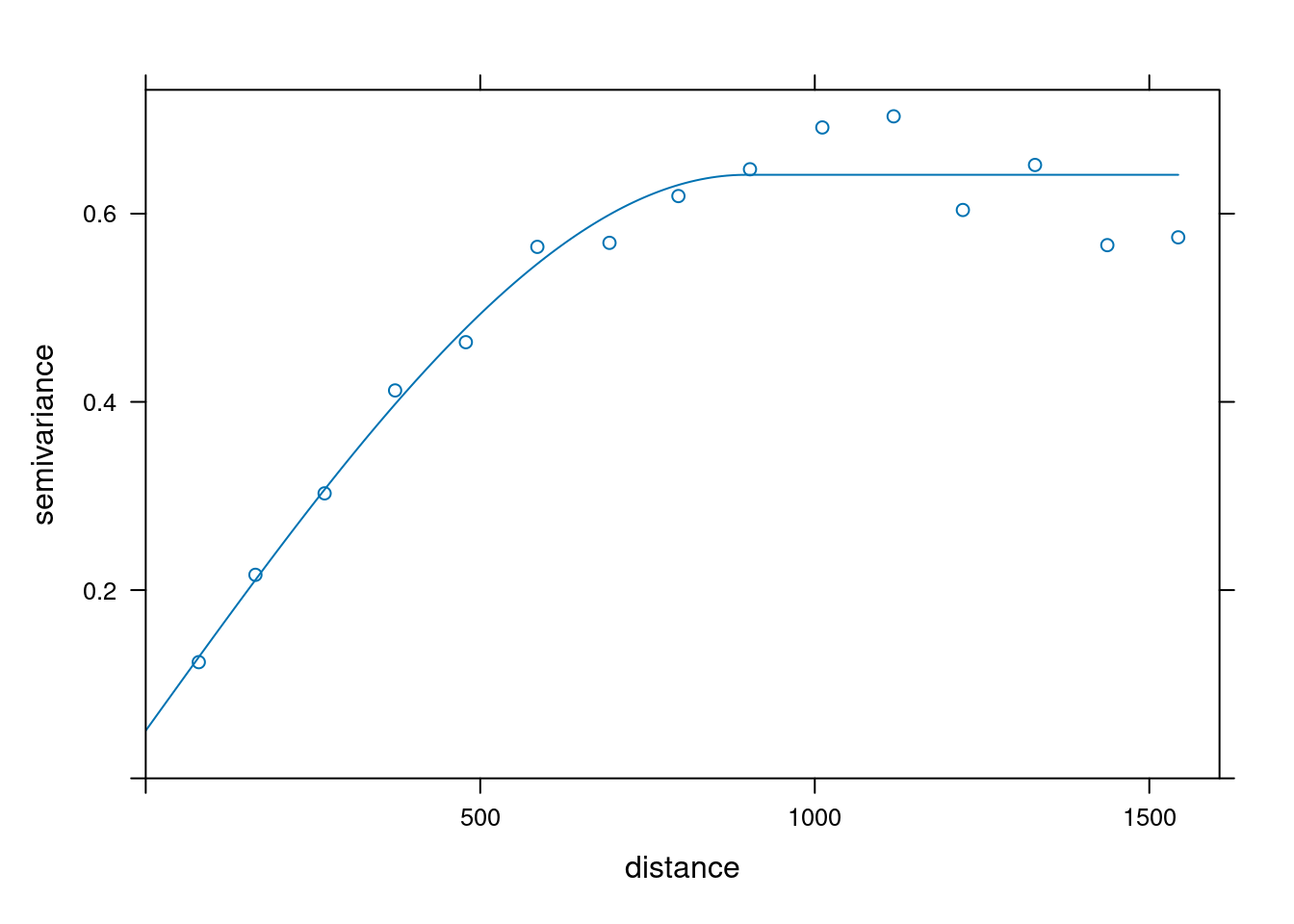
v.fit
#   model  psill range
# 1   Nug 0.0507     0
# 2 Sph 0.5906 897vgm(psill = 0.6, model = "Sph", range = 900, nugget = 0.06)
# model psill range
# 1 Nug 0.06 0
# 2 Sph 0.60 900or simpler, with un-named arguments: ::: {.cell}
vgm(0.6, "Sph", 900, 0.06)
#   model psill range
# 1   Nug  0.06     0
# 2   Sph  0.60   900
:::
Covariance: \(\Cov(Z(s),Z(s+h)) = C(h) = \E[(Z(s)-m)(Z(s+h)-m)]\)
Semivariance: \(\gamma(h) = \frac{1}{2} \E[(Z(s)-Z(s+h))^2]\)
\[\gamma(h)=C(0)-C(h)\]
This is nothing else then simple kriging, except that the mean is no longer constant; BLP/Simple kriging: \[\hat{Z}(s_0) = \mu(s_0) + v'V^{-1} (Z-\mu(s))\] \[\sigma^2(s_0) = \sigma^2_0 - v'V^{-1}v\] with \(\mu(s) = (\mu(s_1),\mu(s_2),...,\mu(s_n))'\).