10  Cokriging, cross validation, conditional simulation

\[ \newcommand{\E}{{\rm E}} % E expectation operator \newcommand{\Var}{{\rm Var}} % Var variance operator \newcommand{\Cov}{{\rm Cov}} % Cov covariance operator \newcommand{\Cor}{{\rm Corr}} \]

10.1 cokriging

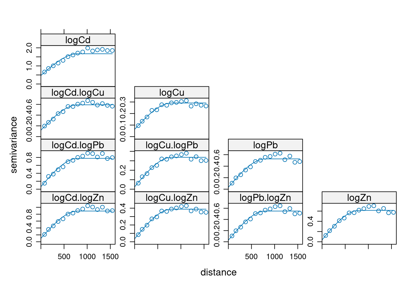
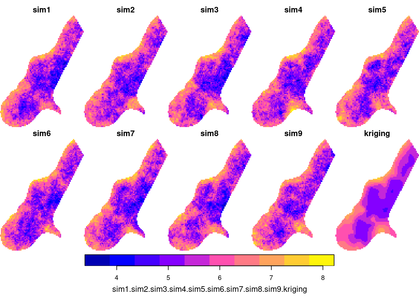
Cokriging sets the multivariate equivalent of kriging, which is, in terms of number of dependent variables, univariate. Kriging: \[Z(s) = X(s)\beta + e(s)\] Cokriging: \[Z_1(s) = X_1(s)\beta_1 + e_1(s)\] \[Z_2(s) = X_2(s)\beta_2 + e_2(s)\] \[Z_k(s) = X_k(s)\beta_k + e_k(s)\] with \(V = \Cov(e_1,e_2,...,e_k)\)

Cases where this is useful: multiple spatial correlated variables such as

  • chemical properties (auto-analyzers!)
  • sediment composition
  • electromagnetic spectra (imagery/remote sensing)
  • ecological data (abiotic factors; species abundances)
  • (space-time data, with discrete time)

Two types of applications:

  • undersampled case: secondary variables help prediction of a primary, because we have more samples of them (image?)
  • equally sampled case: secondary variables don’t help prediction much, but we are interested in multivariate prediction, i.e. prediction error covariances.

Cokriging prediction

Cokriging prediction is not substantially different from kriging prediction, it is just a lot of book-keeping.

How to set up \(Z(s)\), \(X\), \(\beta\), \(e(s)\), \(x(s_0)\), \(v\), \(V\)?

Multivariable prediction involves the joint prediction of multiple, both spatially and cross-variable correlated variables. Consider \(m\) distinct variables, and let \(\{Z_i(s), X_i, \beta^i, e_i(s), x_i(s_0), v_i, V_i\}\) correspond to \(\{Z(s), X, \beta, e(s), x(s_0), v, V\}\) of the \(i\)-th variable. Next, let \({\bf Z}(s) = (Z_1(s)',...,Z_m(s)')'\), \({\bf B}=({\beta^1} ',...,{\beta^m} ')'\), \({\bf e}(s)=(e_1(s)',...,e_m(s)')'\),

\[ {\bf X} = \left[ \begin{array}{cccc} X_1 & 0 & ... & 0 \\\\ 0 & X_2 & ... & 0 \\\\ \vdots & \vdots & \ddots & \vdots \\\\ 0 & 0 & ... & X_m \\\\ \end{array} \right], \ {\bf x}(s_0) = \left[ \begin{array}{cccc} x_1(s_0) & 0 & ... & 0 \\\\ 0 & x_2(s_0) & ... & 0 \\\\ \vdots & \vdots & \ddots & \vdots \\\\ 0 & 0 & ... & x_m(s_0) \\\\ \end{array} \right] \]

with \(0\) conforming zero matrices, and

\[{\bf v} = \left[ \begin{array}{cccc} v_{1,1} & v_{1,2} & ... & v_{1,m} \\\\ v_{2,1} & v_{2,2} & ... & v_{2,m} \\\\ \vdots & \vdots & \ddots & \vdots \\\\ v_{m,1} & v_{m,2} & ... & v_{m,m} \\\\ \end{array} \right], \ \ {\bf V} = \left[ \begin{array}{cccc} V_{1,1} & V_{1,2} & ... & V_{1,m} \\\\ V_{2,1} & V_{2,2} & ... & V_{2,m} \\\\ \vdots & \vdots & \ddots & \vdots \\\\ V_{m,1} & V_{m,2} & ... & V_{m,m} \\\\ \end{array} \right] \]

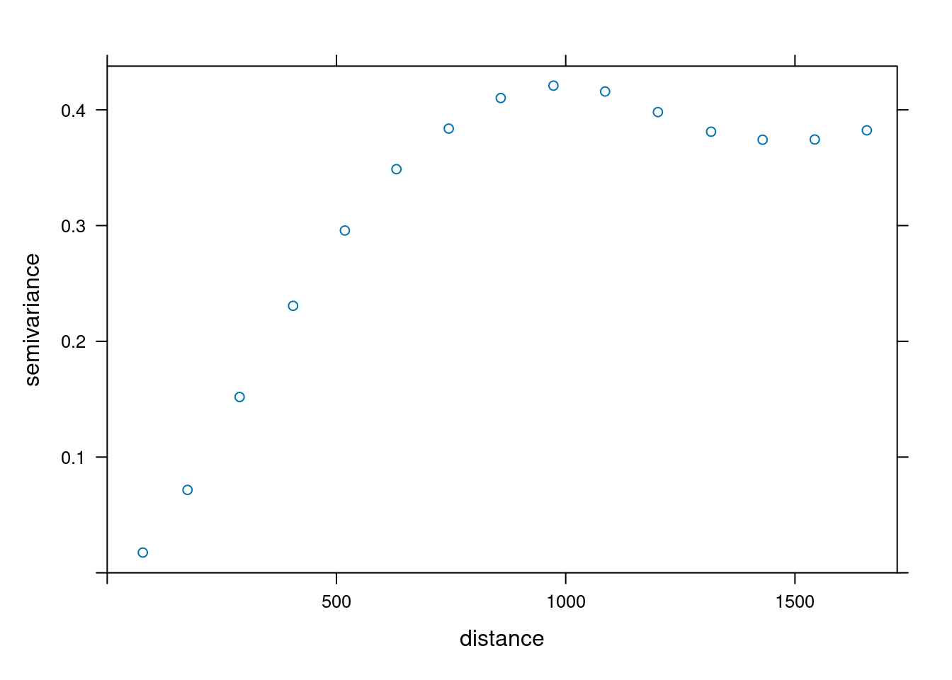
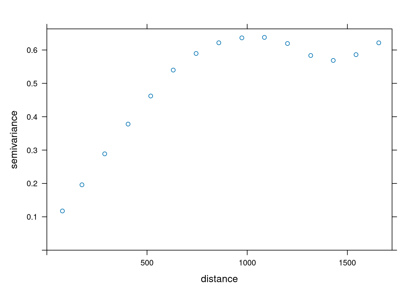
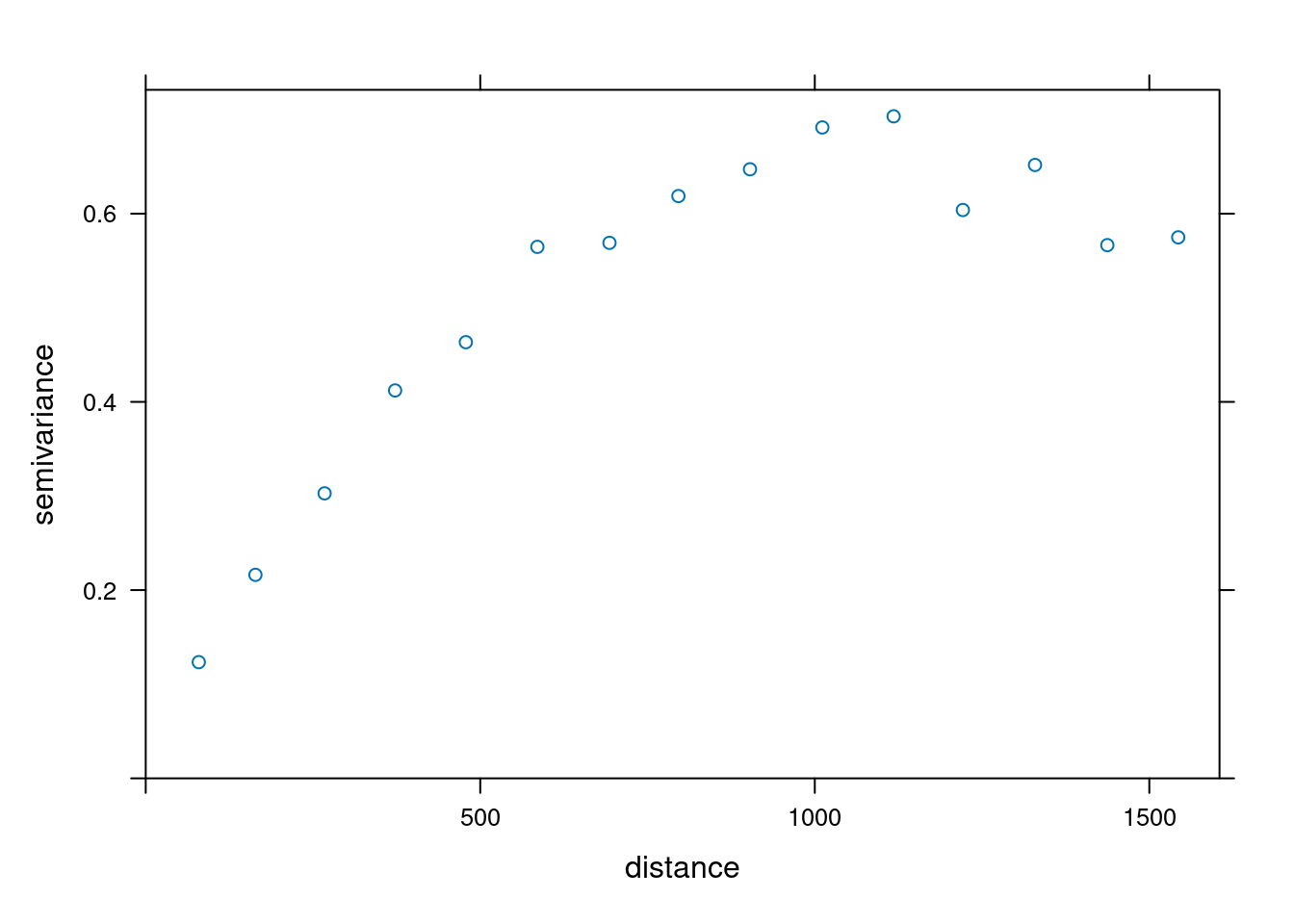
where element \(i\) of \(v_{k,l}\) is \(\Cov(Z_k(s_i), Z_l(s_0))\), and where element \((i,j)\) of \(V_{k,l}\) is \(\Cov(Z_k(s_i),Z_l(s_j))\).

The multivariable prediction equations equal the previous UK equations and when all matrices are substituted by their multivariable forms (see also Ver Hoef and Cressie, Math.Geol., 1993), and when for \(\sigma^2_0\), \(\Sigma\) is substituted with \(\Cov(Z_i(s_0),Z_j(s_0))\) in its \((i,j)\)-th element. Note that the prediction variance is now a prediction error covariance matrix.

What is needed?

The main tool for estimating semivariances between different variables is the cross variogram, defined for collocated data as \[\gamma_{ij}(h) = \mbox{E}[(Z_i(s)-Z_i(s+h))(Z_j(s)-Z_j(s+h))]\] and for non-collocated data as \[\gamma_{ij}(h) = \mbox{E}[(Z_i(s)-m_i)(Z_j(s+h)-m_j)]\] with \(m_i\) and \(m_j\) the means of the respective variables. Sample cross variograms are the obvious sums over the available pairs or cross pairs, as in one of \[\hat{\gamma}_{jk}(\tilde{h})=\frac{1}{N_h}\sum_{i=1}^{N_h}(Z_j(s_i)-Z_j(s_i+h))(Z_k(s_i)-Z_k(s_i+h))\] \[\hat{\gamma}_{jk}(\tilde{h})=\frac{1}{N_h}\sum_{i=1}^{N_h}(Z_j(s_i)-m_j)(Z_k(s_i+h)-m_k)\]

Permissible cross covariance functions

Two classes of permissible cross covariance (semivariance) functions are often used:

  • intrinsic correlation (IC): \[\gamma_{jk}(h) = \alpha_{jk} \sqrt{\gamma_{jj}(h)\gamma_{kk}(h)}\] parameters \(\alpha_{jk}\) are correlation cofficients; very strict
  • linear model of coregionalization (LMC): \[\gamma_{jk}(h) = \sum_{l=1}^p \gamma_{jk,p}(h)\] (e.g., nugget + spherical model), and \[\gamma_{jk,p}(h) = \alpha_{jk,p} \sqrt{\gamma_{jj,p}(h)\gamma_{kk,p}(h)}\]

How to do this?

As multivariable analysis may involve numerous variables, we need to start organising the available information. For that reason, we collect all the observation data specifications in a gstat object, created by the function gstat. This function does nothing else than ordering (and actually, copying) information needed later in a single object. Consider the following definitions of four heavy metals:

library(sf)
library(sp)
library(gstat)
data(meuse, package = "sp")
meuse = st_as_sf(meuse, coords = c("x", "y"))
g <- gstat(id = "logCd", formula = log(cadmium)~1, data = meuse)
g <- gstat(g, "logCu", log(copper)~1, data = meuse)
g <- gstat(g, "logPb", log(lead)~1, data = meuse)
g <- gstat(g, "logZn", log(zinc)~1, data = meuse)
g 
# data:
# logCd : formula = log(cadmium)`~`1 ; data dim = 155 x 12
# logCu : formula = log(copper)`~`1 ; data dim = 155 x 12
# logPb : formula = log(lead)`~`1 ; data dim = 155 x 12
# logZn : formula = log(zinc)`~`1 ; data dim = 155 x 12
vm <- variogram(g)
vm.fit <- fit.lmc(vm, g, vgm(1, "Sph", 800, 1))
plot(vm, vm.fit)

Kriging predictions and errors – how good are they?

Cross validation can be used to assess the quality of any interpolation, including kriging. We split the data set in \(n\) parts (folds). For each part, we

  • leave out the observations of this fold
  • use the observations of all other folds to predict the values at the locations of this fold
  • compare the predictions with the observations This is called \(n\)-fold cross validation. If \(n\) equals the number of observation, it is called leave-one-out cross validation (LOOCV).

Cross validation: what does it yield?

  • residuals \(r(s_i) = z(s_i) -\hat{z}(s_i)\) – histograms, maps, summary statistics
  • mean residual should be near zero
  • mean square residual \(\sum r(s_i)^2\) should be as small as possible

In case the interpolation method yields a prediction error we can compute z-scores: \(r(s_i)/\sigma(s_i)\)

The z-score allows the validation of the kriging error, as the z-score should have mean close to zero and variance close to 1. If the variance of the z-score is larger (smaller) than 1, the kriging standard error is underestimating (overestimating) the true interpolation error, on average.

Kriging errors – what do they mean?

Suppose legislation prescribes remediation in case zinc exceeds 500 ppm. Where does the zinc level exceed 500 ppm?

  • we can compare the map of the predictions with 500. However:
    • \(\hat{z}(s_0)\) does not equal \(z(s_0)\):
    • \(\hat{z}(s_0)\) is more smooth than \(z(s_0)\)
    • \(\hat{z}(s_0)\) is closer to the mean than \(z(s_0)\)
    • smoothing effect is stronger if spatial correlation is small or nugget effect is relatively large
  • alternatively we can assume that the true (unknown) value follows a probability distribution, with mean \(\hat{z}(s_0)\) and standard error \(\sigma(s_0)\).
  • this latter approach acknowledges that \(\sigma(s_0)\) is useful as a measure of interpolation accuracy

Conditional probability

  • we can use e.g. the normal distribution (on the log-scale?) to assess the conditional probability \(\Pr(Z(s_0) > 500 | z(s_1),...,z(s_n))\)
  • the additional assumption underlying this is multivariate normality: in addition to having stationary mean and covariance, the field \(Z\) is now assumed to follow a stationary, multivariate normal distribution. This means that any single \(Z(s_i)\) follows a normal distribution, and any pair \(Z(s_i), Z(s_j)\) follows a bivariate normal distribution, with known variances and covariance.

How?

v = variogram(log(zinc)~1, meuse)
v.fit = fit.variogram(v, vgm(1, "Sph", 900, 1))
data(meuse.grid, package = "sp")
library(stars)
meuse.grid = st_as_stars(meuse.grid)
out = krige(log(zinc)~1, meuse, meuse.grid, v.fit)
# [using ordinary kriging]
out$p500 = 1 - pnorm(log(500), out$var1.pred, sqrt(out$var1.var))
plot(out["p500"], col = sf.colors(), breaks = "equal")

Indicator kriging

Another approach to estimating probabilities of exceedance is to consider the indicator function, which is 1 if a value exceeds the threshold and 0 otherwise:

mean(meuse$zinc)
# [1] 470
mean(meuse$zinc < 500)
# [1] 0.632
v = variogram(I(zinc > 500)~1, meuse)
v_I.fit = fit.variogram(v, vgm(.2, "Sph", 900, .02))
plot(v, v_I.fit)

out$I500 = krige(I(zinc > 500)~1, meuse, meuse.grid, v_I.fit)$var1.pred
# [using ordinary kriging]
out["I500"] # summarizes
# stars object with 2 dimensions and 1 attribute
# attribute(s):
#          Min. 1st Qu. Median  Mean 3rd Qu. Max. NA's
# I500  -0.0876  0.0546  0.193 0.296   0.525 1.03 5009
# dimension(s):
#   from  to offset delta x/y
# x    1  78 178440    40 [x]
# y    1 104 333760   -40 [y]
plot(merge(out[c("p500", "I500")]), col = bpy.colors(), breaks = "equal")

This second approach:

  • ignores the kriging variance
  • generates probabilities outside the interval \([0, 1]\) (to be corrected?)
  • ignores information whether observations are close to the threshold, or far away from it (they are reduced to 1/0 variable before interpolating)
  • does not assume multivariate normality
  • does not distinguish between estimated probabilities and (true) probabilities
  • lends itself to the interpolation of categorical (nominal, ordinal) variables
  • cokriging is sometimes used for interpolating several indicator variables (multiple categories, or multiple thresholds)

Conditional simulation

v = variogram(log(zinc)~1, meuse)
v.fit = fit.variogram(v, vgm(1, "Sph", 900, 1))
out = krige(log(zinc)~1, meuse, meuse.grid, v.fit, nmax = 20, nsim = 9)
# drawing 9 GLS realisations of beta...
# [using conditional Gaussian simulation]
out = split(out)
out$kriging = krige(log(zinc)~1, meuse, meuse.grid, v.fit)$var1.pred
# [using ordinary kriging]
plot(merge(out), col = sf.colors(), breaks = "equal")

sf = st_as_sf(out, as_points = TRUE)
v_kr = variogram(kriging~1, sf)
v_cs = variogram(sim1~1, sf)
plot(v_kr)

plot(v_cs)

plot(v)

  • conditional simulation creates multiple realisations of the field \(Z(s)\) that
    • follow the data points (pattern, reproduce observations like kriging)
    • have a variability equal to Z(s)
    • have a spatial correlation (variogram) equal to that of Z(s)
  • as opposed to kriging, the resulting images are not smooth
  • this is useful e.g. if images are needed as input to subsequent processing / modelling, where the statistical properties of Z(s) need to be retained (e.g. simulating rainfall fields as input to rainfall-runoff models, to predict the likelihood of flooding / extreme water levels)