
st_is_simple(x1)
# [1] FALSE
st_is_simple(x2)
# [1] FALSE(thanks to Jannis Fröhlking)
Give two examples of geometries in 2-D (flat) space that are not simple feature geometries, and create a plot of them.
Recompute the coordinates 10.542, 0.01, 45321.789 using precision values 1, 1e3, 1e6, and 1e-2.
Describe a practical problem for which an n-ary intersection would be needed.
How can you create a Voronoi diagram (figure 3.3) that has closed polygons for every point?
Voronoi diagrams have “open polygons”, areas that extend into infinity, for boundary points. These cannot be represented by simple feature geometries. st_voronoi chooses a default (square) polygon to limit the extent, which can be enlarged. Alternatively, the extent can be limited using st_intersection on its result:
library(sf)
par(mfrow = c(2,2))
set.seed(133331)
mp = st_multipoint(matrix(runif(20), 10))
plot(st_voronoi(mp), col = NA, border = 'black')
plot(mp, add = TRUE)
title("default extent")
e2 = st_polygon(list(rbind(c(-5,-5), c(5, -5), c(5,5), c(-5, 5), c(-5,-5))))
plot(st_voronoi(mp, envelope = e2), col = NA, border = 'black')
plot(mp, add = TRUE)
title("enlarged envelope")
e3 = st_polygon(list(rbind(c(0,0), c(1, 0), c(1, 1), c(0, 1), c(0, 0))))
v = st_voronoi(mp) |> st_collection_extract() # pulls POLYGONs out of GC
plot(st_intersection(v, e3), col = NA, border = 'black', axes=TRUE)
plot(mp, add = TRUE)
title("smaller, intersected envelope")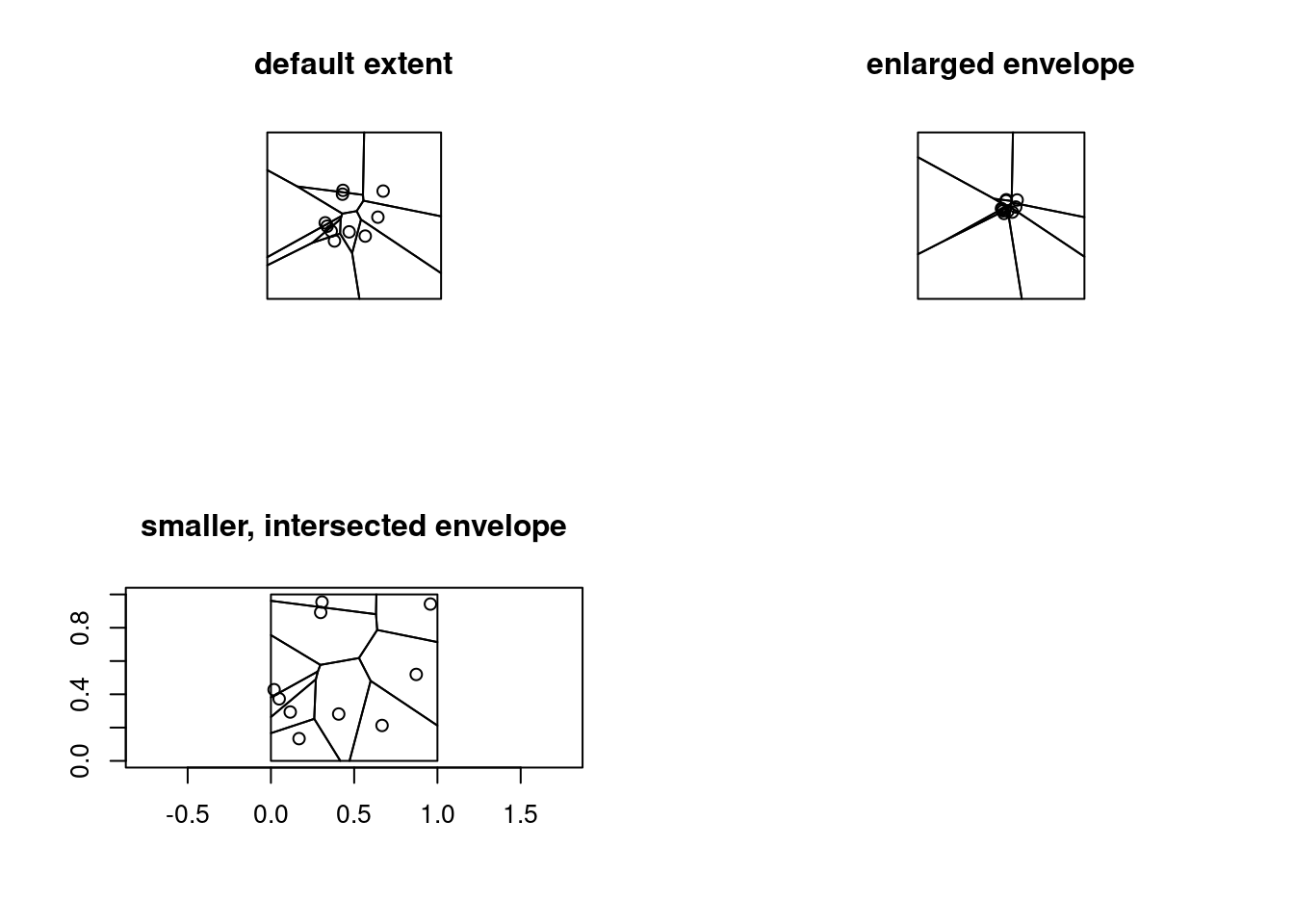
Give the unary measure dimension for geometries POINT Z (0 1 1), LINESTRING Z (0 0 1,1 1 2), and POLYGON Z ((0 0 0,1 0 0,1 1 0,0 0 0))
st_dimension(st_point(c(0,1,1)))
# [1] 0
st_dimension(st_linestring(rbind(c(0,1,1),c(1,1,2))))
# [1] 1
st_dimension(st_polygon(list(rbind(c(0,0,0),c(1,0,0),c(1,1,0),c(0,0,0)))))
# [1] 2
(these are all zero-dimensional geometries because they are points, irrespective the number of dimensions they’re defined in)
Give the DE-9IM relation between LINESTRING(0 0,1 0) and LINESTRING(0.5 0,0.5 1); explain the individual characters.
line_1 = st_linestring(rbind(c(0,0),c(1,0)))
line_2 = st_linestring(rbind(c(.5,0),c(.5,1)))
plot(line_1,col = "green")
plot(line_2,col = "red", add = TRUE)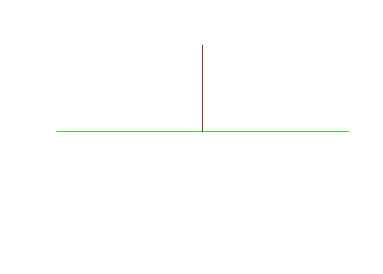
st_relate(line_1, line_2)
#      [,1]
# [1,] "F01FF0102"
The DE-9IM relation is F01FF0102
(the boundary of a LINESTRING is formed by its two end points)
Can a set of simple feature polygons form a coverage? If so, under which constraints? Yes, but I would say that the set may just contain one polygon, because simple features provide no way of assigning points on the boundary of two adjacent polygons to a single polygon.
For the nc counties in the dataset that comes with R package sf, find the points touched by four counties.
# read data
nc <- st_read(system.file("shape/nc.shp", package="sf"))
# Reading layer `nc' from data source
#   `/home/edzer/R/x86_64-pc-linux-gnu-library/4.4/sf/shape/nc.shp'
#   using driver `ESRI Shapefile'
# Simple feature collection with 100 features and 14 fields
# Geometry type: MULTIPOLYGON
# Dimension:     XY
# Bounding box:  xmin: -84.32385 ymin: 33.88199 xmax: -75.45698 ymax: 36.58965
# Geodetic CRS:  NAD27
# get intersections
(nc_geom = st_geometry(nc))
# Geometry set for 100 features
# Geometry type: MULTIPOLYGON
# Dimension:     XY
# Bounding box:  xmin: -84.32385 ymin: 33.88199 xmax: -75.45698 ymax: 36.58965
# Geodetic CRS:  NAD27
# First 5 geometries:
# MULTIPOLYGON (((-81.47276 36.23436, -81.54084 3...
# MULTIPOLYGON (((-81.23989 36.36536, -81.24069 3...
# MULTIPOLYGON (((-80.45634 36.24256, -80.47639 3...
# MULTIPOLYGON (((-76.00897 36.3196, -76.01735 36...
# MULTIPOLYGON (((-77.21767 36.24098, -77.23461 3...
nc_ints = st_intersection(nc_geom)
# although coordinates are longitude/latitude, st_intersection
# assumes that they are planar
plot(nc_ints, main = "All intersections")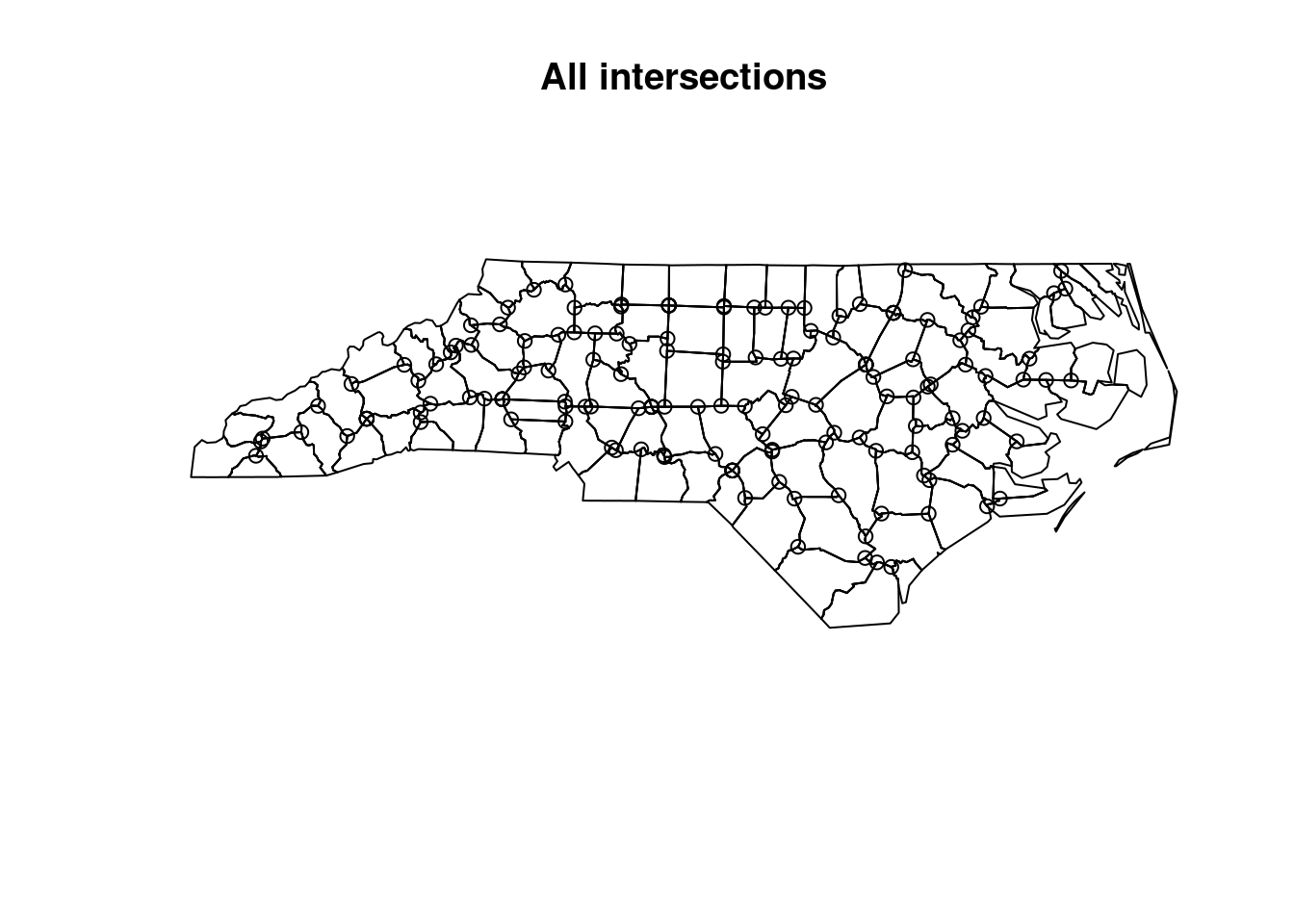
# Function to check class of intersection objects
get_points = function(x){
  if(class(x)[2]=="POINT")  return(x)
}
# get points
points = lapply(nc_ints, get_points)
points[sapply(points,is.null)] <- NULL
sf_points = st_sfc(points)
st_crs(sf_points) = st_crs(nc)
# get points with four neighbouring geometries (=states)
touch = st_touches(sf_points, nc_geom)
four_n = sapply(touch, function(y) which(length(y)==4))
names(four_n) = seq_along(four_n)
point_no = array(as.numeric(names(unlist(four_n))))
result = st_sfc(points[point_no])
plot(nc_geom, main = "Points touched by four counties")
plot(result, add = TRUE, col = "red", pch = 10, cex = 2)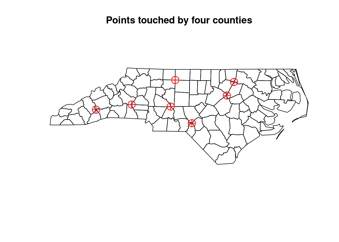
A more compact way might be to search for points where counties touch another county only in a point, which can be found using st_relate using a pattern:
(pts = nc |> st_relate(pattern = "****0****"))
# although coordinates are longitude/latitude, st_relate_pattern
# assumes that they are planar
# Sparse geometry binary predicate list of length 100, where
# the predicate was `relate_pattern'
# first 10 elements:
#  1: (empty)
#  2: (empty)
#  3: (empty)
#  4: (empty)
#  5: (empty)
#  6: (empty)
#  7: (empty)
#  8: (empty)
#  9: 31
#  10: 26
nc |> st_relate(pattern = "****0****") |> lengths() |> sum()
# although coordinates are longitude/latitude, st_relate_pattern
# assumes that they are planar
# [1] 28
which is, as expected, four times the number of points shown in the plot above.
How can we find these points? See here:
nc = st_geometry(nc)
s2 = sf_use_s2(FALSE) # use GEOM geometry
# Spherical geometry (s2) switched off
pts = st_intersection(nc, nc)
# although coordinates are longitude/latitude, st_intersection
# assumes that they are planar
pts = pts[st_dimension(pts) == 0]
plot(st_geometry(nc))
plot(st_geometry(pts), add = TRUE, col = "red", pch = 10, cex = 2)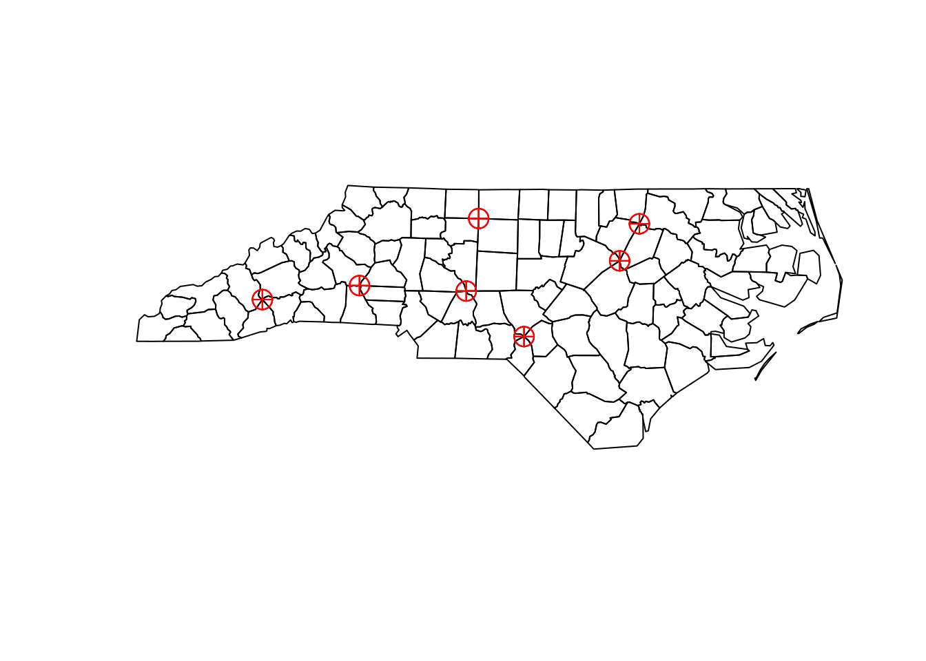
sf_use_s2(s2) # set back
# Spherical geometry (s2) switched onHow would figure 3.6 look like if delta for the y-coordinate was positive? Only cells that were fully crossed by the red line would be grey:
library(stars)
# Loading required package: abind
ls = st_sf(a = 2, st_sfc(st_linestring(rbind(c(0.1, 0), c(1, .9)))))
grd = st_as_stars(st_bbox(ls), nx = 10, ny = 10, xlim = c(0, 1.0), ylim = c(0, 1),
   values = -1)
attr(grd, "dimensions")$y$delta = .1
attr(grd, "dimensions")$y$offset = 0
r = st_rasterize(ls, grd, options = "ALL_TOUCHED=TRUE")
r[r == -1] = NA
plot(st_geometry(st_as_sf(grd)), border = 'orange', col = NA,
     reset = FALSE, key.pos=NULL)
plot(r, axes = TRUE, add = TRUE, breaks = "equal") # ALL_TOUCHED=FALSE;
plot(ls, add = TRUE, col = "red", lwd = 2)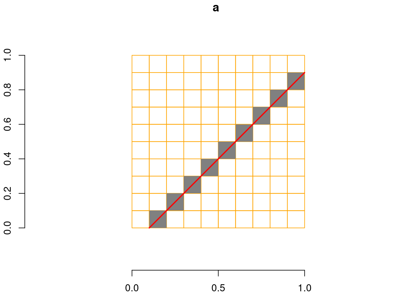
The reason is that in this case, lower left corners of grid cells are part of the cell, rather than upper left corners.