11  Spatial Point Patterns

Exercise 11.1

After loading spatstat, recreate the plot obtained by plot(longleaf) by using ggplot2 and geom_sf(), and by sf::plot().

library(spatstat)
# Loading required package: spatstat.data
# Loading required package: spatstat.geom
# spatstat.geom 3.2-9
# Loading required package: spatstat.random
# spatstat.random 3.2-3
# Loading required package: spatstat.explore
# Loading required package: nlme
# spatstat.explore 3.2-7
# Loading required package: spatstat.model
# Loading required package: rpart
# spatstat.model 3.2-11
# Loading required package: spatstat.linnet
# spatstat.linnet 3.1-5
# 
# spatstat 3.0-8 
# For an introduction to spatstat, type 'beginner'
library(sf)
# Linking to GEOS 3.10.2, GDAL 3.4.1, PROJ 8.2.1; sf_use_s2() is TRUE
plot(longleaf) # spatstat plot

# using sf::plot() :
ll = st_as_sf(longleaf)
box = ll[1,]
pts = ll[-1,]
st_geometry(box) |> plot() #cex = 2*marks/max(marks))
marks = pts$spatstat.geom..marks.x
st_geometry(pts) |> plot(cex = 2*marks/max(marks), add = TRUE)

# using ggplot2:
library(ggplot2)
pts$marks = marks
ggplot() + geom_sf(data = box) + geom_sf(data = pts, aes(size = marks))

# how to get open circles? use geom_point():
p = as.data.frame(st_coordinates(pts))
ggplot() + geom_sf(data = box) + geom_point(aes(x = X, y = Y), data = p, shape = 1, size = 10 * marks / max(marks))

Exercise 11.2

Convert the sample locations of the NO\(_2\) data used in Chapter 12 to a ppp object, with a proper window.

library(tidyverse) |> suppressPackageStartupMessages()
no2 <- read_csv(system.file("external/no2.csv", 
    package = "gstat"), show_col_types = FALSE)
library(sf)
crs <- st_crs("EPSG:32632")
st_as_sf(no2, crs = "OGC:CRS84", coords = 
    c("station_longitude_deg", "station_latitude_deg")) |>
    st_transform(crs) -> no2.sf
# read_sf("data/de_nuts1.gpkg") |> st_transform(crs) -> de
"https://github.com/edzer/sdsr/raw/main/data/de_nuts1.gpkg" |> 
  read_sf() |> 
  st_transform(crs) -> de
# create an observation window sf object that contains the same mark:
win = st_sf(NO2 = NA, geometry = st_union(st_geometry(de)))
rbind(win, no2.sf[,"NO2"]) |> as.ppp() -> p
plot(p)

Alternatively, the ppp object can be created stepwise:

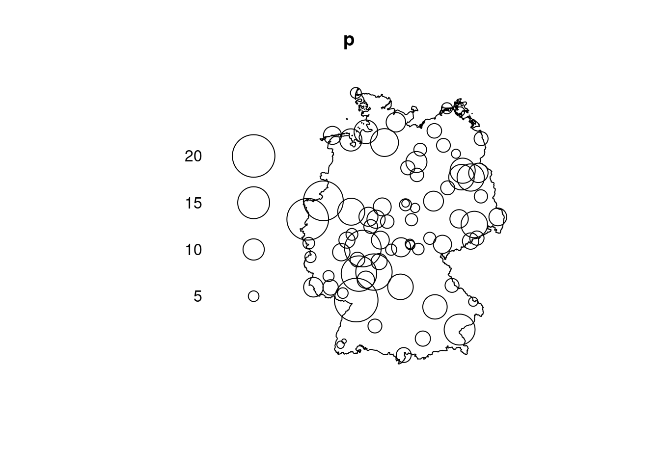
st_union(st_geometry(de)) |> as.owin() -> w
st_geometry(no2.sf) |> as.ppp(W = w) -> p # requires sf 1.0-9
marks(p) = no2.sf$NO2
p
# Marked planar point pattern: 74 points
# marks are numeric, of storage type  'double'
# window: polygonal boundary
# enclosing rectangle: [280741.3, 921330.5] x [5235822, 6101239] 
# units

Exercise 11.3

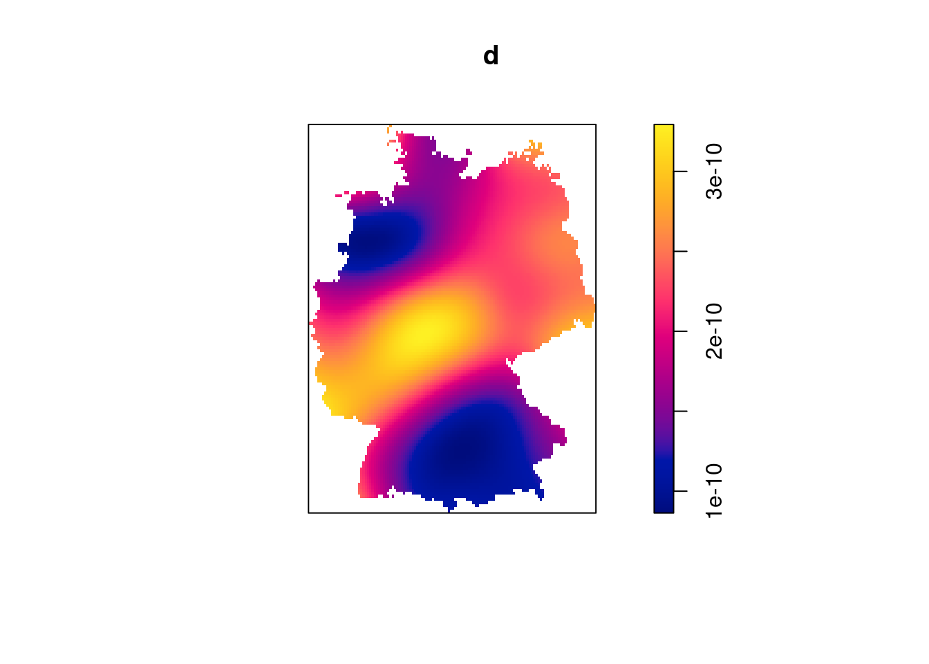
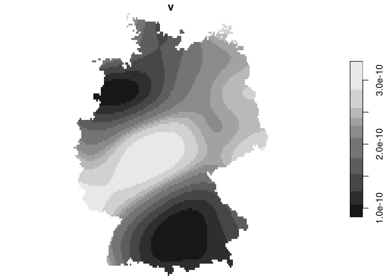
Compute and plot the density of the NO\(_2\) dataset, import the density as a stars object and compute the volume under the surface.

d = density(p)
plot(d)

library(stars)
# Loading required package: abind
st_as_stars(d) |> st_set_crs(crs) -> s
plot(s)

mean(s[[1]], na.rm = TRUE) * st_area(win)
# 71.06103 [m^2]

this number is close to the number of observations,

nrow(no2.sf)
# [1] 74