Why is it difficult to represent trajectories, sequences of \((x,y,t)\) obtained by tracking moving objects, by data cubes as described in this chapter?
rounding \((x,y,t)\) to the discrete set of dimension values in a data cube may cause loss of information
if the dimensions all have a high resolution, data loss is limited but the data cube will be very sparse; this will only be effective if a system capable of storing sparse data cubes is used (e.g. SciDB, TileDB)
Exercise 6.2.
In a socio-economic vector data cube with variables population, life expectancy, and gross domestic product ordered by dimensions country and year, which variables have block support for the spatial dimension, and which have block support for the temporal dimension?
population has spatial block support (total over an area), typically not temporal block support (but the population e.g. on a particular day of the year)
life expectancy is calculated over the total population of the country, and as such has spatial block support; it has temporal block support as the number of deaths over a particular period are counted, it is not clear whether this always corresponds to a single year or a longer period.
GDP has both spatial and temporal block support: it is a total over an area and a time period.
Exercise 6.3.
The Sentinel-2 satellites collect images in 12 spectral bands; list advantages and disadvantages to represent them as (i) different data cubes, (ii) a data cube with 12 attributes, one for each band, and (iii) a single attribute data cube with a spectral dimension.
as (i): it would be easy to cope with the differences in cell sizes;
as (ii): one would have to cope with differences in cell sizes (10, 20, 60m), and it would not be easy to consider the spectral reflectance curve of individual pixels
as (iii): as (ii) but it would be easier to consider (analyse, classify, reduce) spectral reflectance curves, as they are now organized in a dimension
Exercise 6.4.
Explain why a curvilinear raster as shown in figure 1.5 can be considered a special case of a data cube.
Curvilinear grids do not have a simple relationship between dimension index (row/col, i/j) to coordinate values (lon/lat, x/y): one needs both row and col to find the coordinate pair, and from a coordinate pair a rather complex look-up to find the corresponding row and column.
Exercise 6.5.
Explain how the following problems can be solved with data cube operations filter, apply, reduce and/or aggregate, and in which order. Also mention for each which function is applied, and what the dimensionality of the resulting data cube is (if any):
Exercise 6.5.1
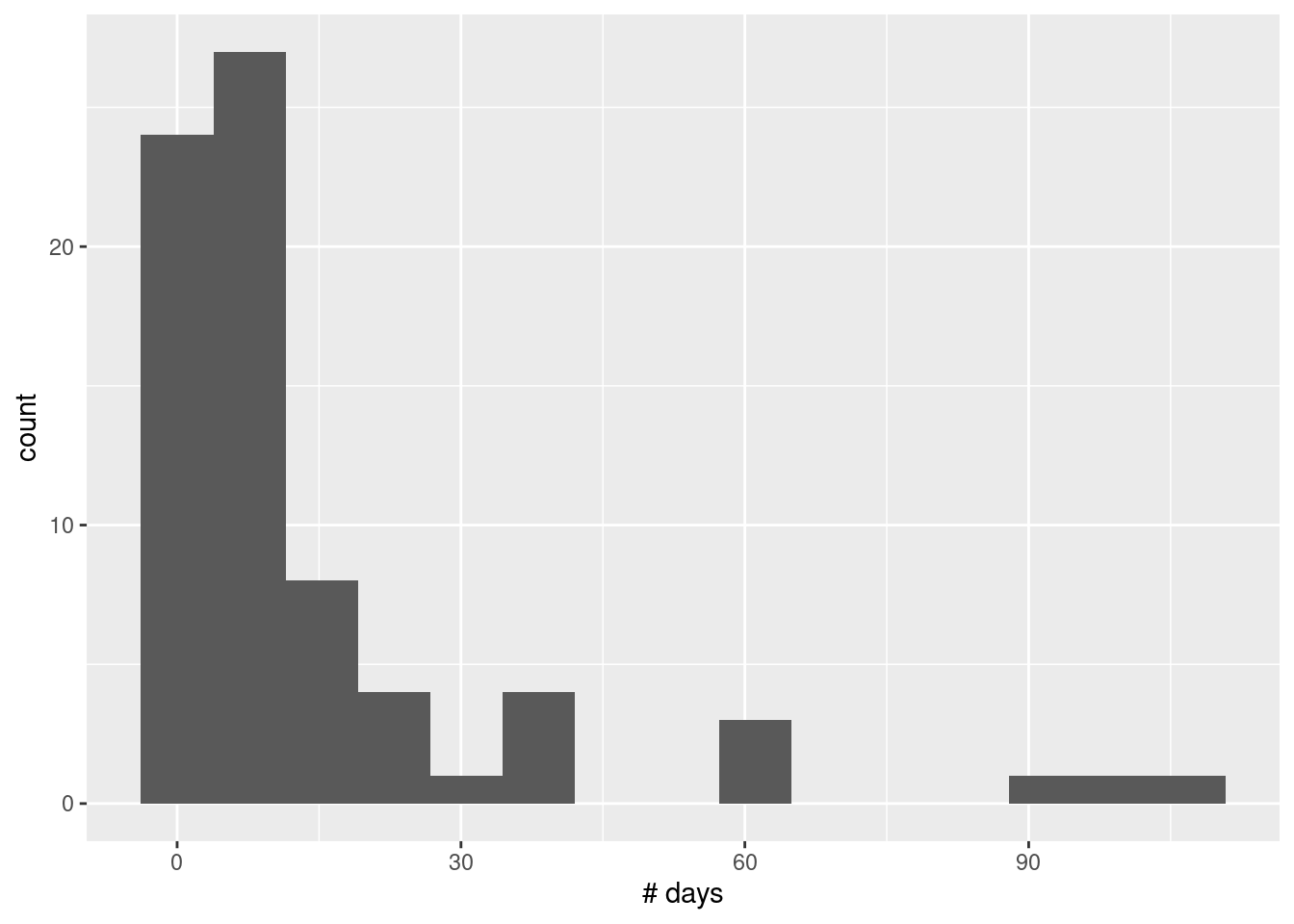
from hourly \(PM_{10}\) measurements for a set of air quality monitoring stations, compute per station the amount of days per year that the average daily \(PM_{10}\) value exceeds 50 \(\mu g/m^3\)
convert measured hourly values into daily averages: aggregate (from hourly to daily, aggregation function: mean)
convert daily averages into TRUE/FALSE whether the daily average exceeds 50: apply (function: larger-than)
compute the number of days: aggregate time to year (aggregation function: sum)
This gives a one-dimensional data cube, with dimension “station”
An example for NO2, 2017, using threshold 25, is given below:
for a sequence of aerial images of an oil spill, find the time at which the oil spill had its largest extent, and the corresponding extent
for each image, classify pixels into oil/no oil: apply (function: classify)
for each image, compute size (extent) of oil spill: reduce space (function: sum)
for the extent time series, find time of maximum: reduce time (function: which.max, then look up time)
This gives a zero-dimensional data cube (a scalar).
Exercise 6.5.3
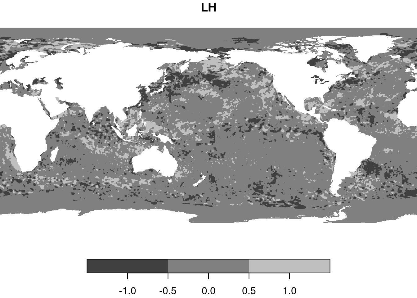
from a 10-year period with global daily sea surface temperature (SST) raster maps, find the area with the 10% largest and 10% smallest temporal trends in SST values.
from daily SST to trend values per pixel: reduce time (function: trend function, lm)
from trend raster, find 10- and 90-percentile: reduce space (function: quantile)
using percentiles, threshold the trend raster: apply (function: less than / more than)
This gives a two-dimensional data cube (or raster layer: the reclassified trend raster).
An example for SST using only a 9-day time series:
Code
library(stars)x=c("avhrr-only-v2.19810901.nc","avhrr-only-v2.19810902.nc","avhrr-only-v2.19810903.nc","avhrr-only-v2.19810904.nc","avhrr-only-v2.19810905.nc","avhrr-only-v2.19810906.nc","avhrr-only-v2.19810907.nc","avhrr-only-v2.19810908.nc","avhrr-only-v2.19810909.nc")# see the second vignette; install with:# options(timeout = 3600)# install.packages("starsdata", repos = "https://cran.uni-muenster.de/pebesma", type = "source")'file_list=system.file(paste0("netcdf/", x), package ="starsdata")l=lapply(file_list, read_stars)# sst, anom, err, ice, # sst, anom, err, ice, # sst, anom, err, ice, # sst, anom, err, ice, # sst, anom, err, ice, # sst, anom, err, ice, # sst, anom, err, ice, # sst, anom, err, ice, # sst, anom, err, ice,do.call(c, append(l, list(along ="time")))|>adrop()->yy# stars object with 3 dimensions and 4 attributes# attribute(s), summary of first 1e+05 cells:# Min. 1st Qu. Median Mean 3rd Qu. Max. NAs# sst [°*C] -1.80 -1.19 -1.05 -0.3201670 -0.20 9.36 13360# anom [°*C] -4.69 -0.06 0.52 0.2299385 0.71 3.70 13360# err [°*C] 0.11 0.30 0.30 0.2949421 0.30 0.48 13360# ice [percent] 0.01 0.73 0.83 0.7657695 0.87 1.00 27377# dimension(s):# from to offset delta x/y# x 1 1440 0 0.25 [x]# y 1 720 90 -0.25 [y]# time 1 9 NA NA# compute trend:lm1=function(y){X=cbind(1, 1:9)if(any(is.na(y)))NA_real_elselm.fit(X,y)$coefficients[2]}tr=st_apply(y[1], c("x","y"), lm1)# find .1 and .9 quantile:qq=quantile(as.vector(tr[[1]]), c(.1, .9), na.rm =TRUE)tr$LH=tr$lm1*0tr$LH[tr$lm1<qq[1]]=-1# lower than .1-quantiletr$LH[tr$lm1>qq[2]]=1# above .9-quantileplot(tr["LH"])