10  Statistical models for spatial data

Exercise 10.1

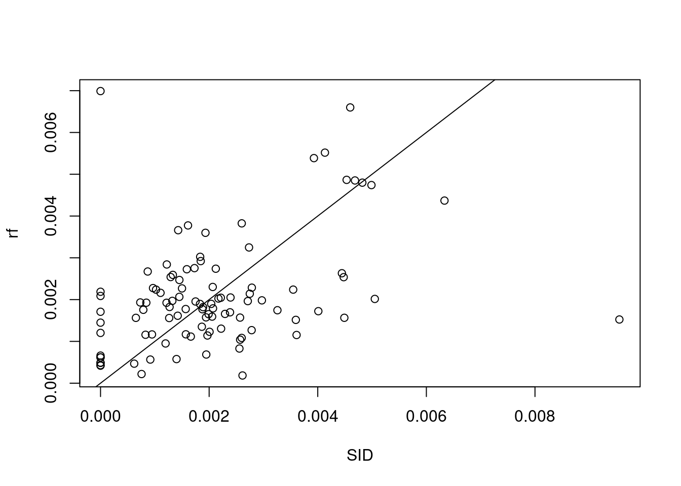
following the lm example of Section 10.2 use a random forest model to predict SID values (e.g. using package randomForest), and plot the random forest predictions against observations, along with the \(x=y\) line.

library(tidyverse)
# ── Attaching core tidyverse packages ──────────── tidyverse 2.0.0 ──
# ✔ dplyr     1.1.4     ✔ readr     2.1.5
# ✔ forcats   1.0.1     ✔ stringr   1.6.0
# ✔ ggplot2   4.0.0     ✔ tibble    3.3.0
# ✔ lubridate 1.9.4     ✔ tidyr     1.3.1
# ✔ purrr     1.2.0     
# ── Conflicts ────────────────────────────── tidyverse_conflicts() ──
# ✖ dplyr::filter() masks stats::filter()
# ✖ dplyr::lag()    masks stats::lag()
# ℹ Use the conflicted package (<http://conflicted.r-lib.org/>) to force all conflicts to become errors
library(sf)
# Linking to GEOS 3.12.1, GDAL 3.8.4, PROJ 9.4.0; sf_use_s2() is TRUE
system.file("gpkg/nc.gpkg", package="sf") |>
    read_sf() -> nc
nc |> mutate(SID = SID74/BIR74, NWB = NWBIR74/BIR74) -> nc1
library(randomForest) |> suppressPackageStartupMessages()
r = randomForest(SID ~ NWB, nc1)
nc1$rf = predict(r)
plot(rf~SID, nc1)
abline(0, 1)

Exercise 10.2

Create a new dataset by randomly sampling 1000 points from the nc dataset, and rerun the linear regression model of section 10.2 on this dataset. What has changed?

pts = st_sample(nc, 1000)
nc2 = st_intersection(nc1, pts)
# Warning: attribute variables are assumed to be spatially constant
# throughout all geometries
lm(SID ~ NWB, nc1) |> summary()
# 
# Call:
# lm(formula = SID ~ NWB, data = nc1)
# 
# Residuals:
#        Min         1Q     Median         3Q        Max 
# -0.0033253 -0.0007411 -0.0000691  0.0005479  0.0062218 
# 
# Coefficients:
#              Estimate Std. Error t value Pr(>|t|)    
# (Intercept) 0.0006773  0.0002327   2.910  0.00447 ** 
# NWB         0.0043785  0.0006204   7.058 2.44e-10 ***
# ---
# Signif. codes:  0 '***' 0.001 '**' 0.01 '*' 0.05 '.' 0.1 ' ' 1
# 
# Residual standard error: 0.001288 on 98 degrees of freedom
# Multiple R-squared:  0.337,   Adjusted R-squared:  0.3302 
# F-statistic: 49.82 on 1 and 98 DF,  p-value: 2.438e-10
lm(SID ~ NWB, nc2) |> summary()
# 
# Call:
# lm(formula = SID ~ NWB, data = nc2)
# 
# Residuals:
#        Min         1Q     Median         3Q        Max 
# -0.0034871 -0.0008685 -0.0001174  0.0005975  0.0060595 
# 
# Coefficients:
#              Estimate Std. Error t value Pr(>|t|)    
# (Intercept) 6.666e-04  8.064e-05   8.266  4.4e-16 ***
# NWB         4.664e-03  2.129e-04  21.903  < 2e-16 ***
# ---
# Signif. codes:  0 '***' 0.001 '**' 0.01 '*' 0.05 '.' 0.1 ' ' 1
# 
# Residual standard error: 0.001364 on 998 degrees of freedom
# Multiple R-squared:  0.3246,  Adjusted R-squared:  0.324 
# F-statistic: 479.7 on 1 and 998 DF,  p-value: < 2.2e-16

we see that the standard error has decreased with a factor 3 (sqrt(10)).

For prediction interval widths:

lm(SID ~ NWB, nc1) |>
  predict(nc1, interval = "prediction") -> pr1
lm(SID ~ NWB, nc2) |>
  predict(nc1, interval = "prediction") -> pr2
mean(pr1[,"upr"] - pr1[,"lwr"])
# [1] 0.005161177
mean(pr2[,"upr"] - pr2[,"lwr"])
# [1] 0.005360656

no change, as this dominated by the residual variance;

Confidence intervals for the predicted means:

lm(SID ~ NWB, nc1) |>
  predict(nc1, interval = "confidence") -> pr1
lm(SID ~ NWB, nc2) |>
  predict(nc1, interval = "confidence") -> pr2
mean(pr1[,"upr"] - pr1[,"lwr"])
# [1] 0.0007025904
mean(pr2[,"upr"] - pr2[,"lwr"])
# [1] 0.0002354517

drops for larger dataset, as this is dominated by the standard errors of estimated coefficients.

Exercise 10.3

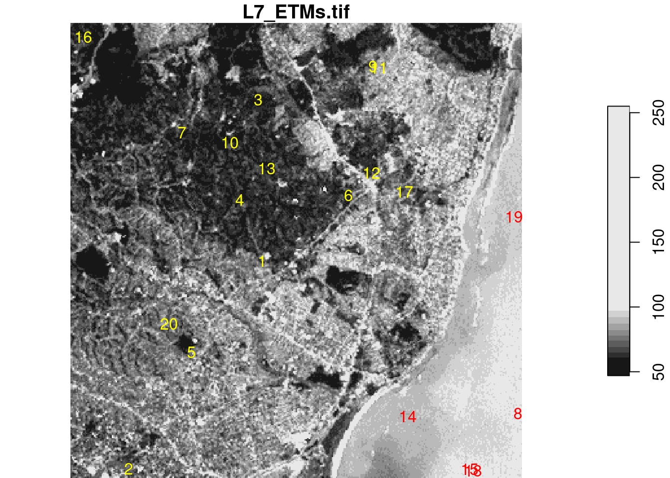
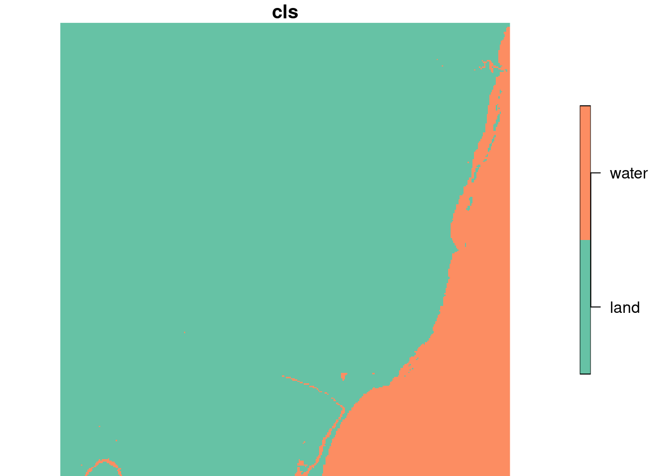
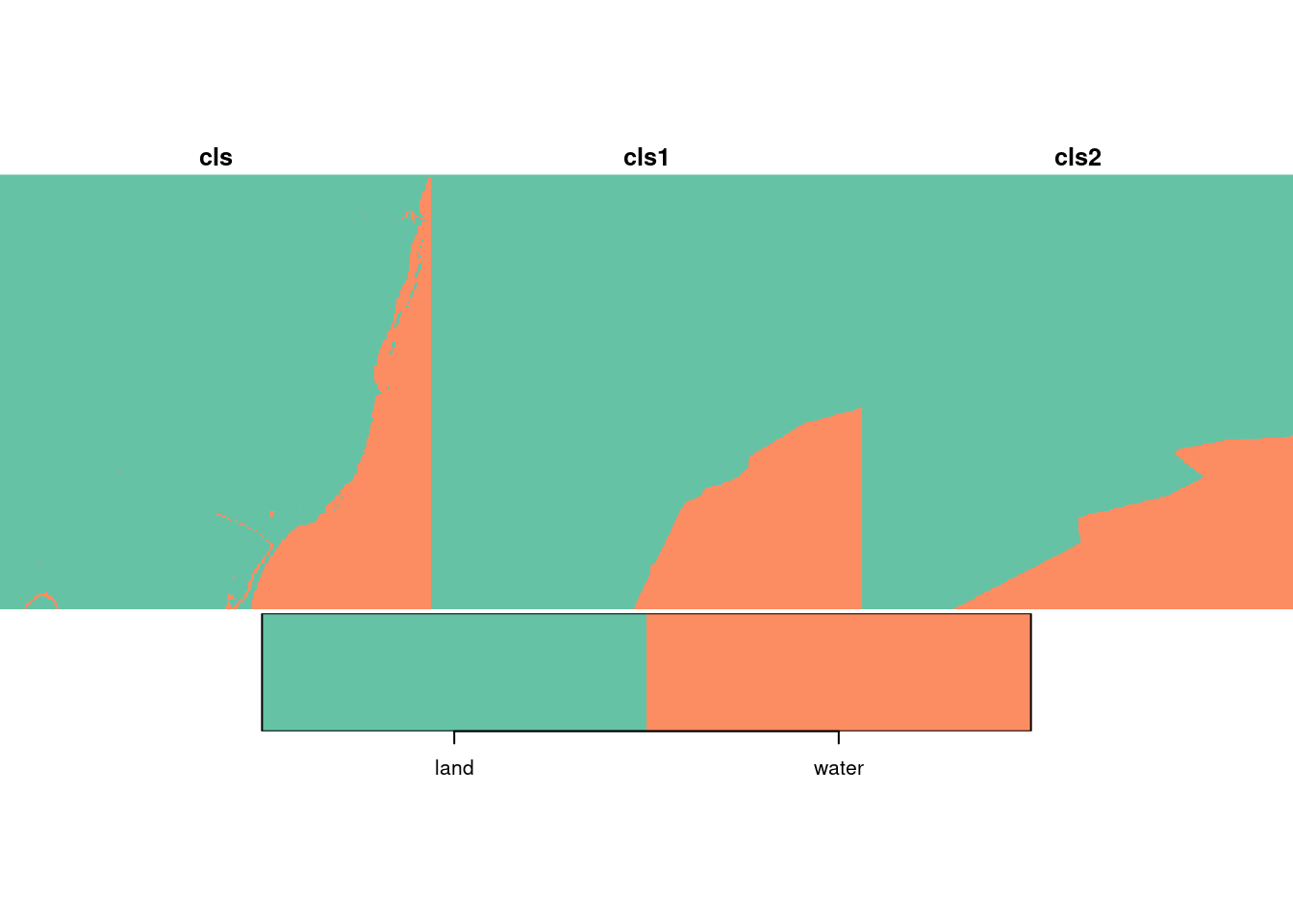
Redo the water-land classification of section 7.4 using class::knn instead of lda.

Preparing the dataset:

tif <- system.file("tif/L7_ETMs.tif", package = "stars")
library(stars)
# Loading required package: abind
(r <- read_stars(tif))
# stars object with 3 dimensions and 1 attribute
# attribute(s):
#              Min. 1st Qu. Median     Mean 3rd Qu. Max.
# L7_ETMs.tif     1      54     69 68.91242      86  255
# dimension(s):
#      from  to  offset delta            refsys point x/y
# x       1 349  288776  28.5 SIRGAS 2000 / ... FALSE [x]
# y       1 352 9120761 -28.5 SIRGAS 2000 / ... FALSE [y]
# band    1   6      NA    NA                NA    NA
set.seed(115517)
pts <- st_bbox(r) |> st_as_sfc() |> st_sample(20)
(e <- st_extract(r, pts))
# stars object with 2 dimensions and 1 attribute
# attribute(s):
#              Min. 1st Qu. Median     Mean 3rd Qu. Max.
# L7_ETMs.tif    12   41.75     63 60.95833    80.5  145
# dimension(s):
#          from to            refsys point
# geometry    1 20 SIRGAS 2000 / ...  TRUE
# band        1  6                NA    NA
#                                           values
# geometry POINT (293002....,...,POINT (290941....
# band                                        NULL
plot(r[,,,1], reset = FALSE)
col <- rep("yellow", 20)
col[c(8, 14, 15, 18, 19)] = "red"
st_as_sf(e) |> st_coordinates() |> text(labels = 1:20, col = col)

rs <- split(r)
trn <- st_extract(rs, pts)
trn$cls <- rep("land", 20)
trn$cls[c(8, 14, 15, 18, 19)] <- "water"

estimation and prediction happen in one command:

library(class)
as.data.frame(trn) |> select(X1, X2, X3, X4, X5, X6) -> tr 
as.data.frame(rs) |> select(X1, X2, X3, X4, X5, X6) -> test
rs$cls = knn(tr, test, trn$cl, k = 5)
plot(rs["cls"])

Exercise 10.4

For the nc data: estimation

st_centroid(nc1) |> st_coordinates() -> cc
# Warning: st_centroid assumes attributes are constant over
# geometries
bind_cols(nc1, cc) |> transmute(X=X, Y=Y, SID=SID, NWB=NWB) -> nc2
(lm0 <- lm(SID ~ NWB, nc1)) |> summary()
# 
# Call:
# lm(formula = SID ~ NWB, data = nc1)
# 
# Residuals:
#        Min         1Q     Median         3Q        Max 
# -0.0033253 -0.0007411 -0.0000691  0.0005479  0.0062218 
# 
# Coefficients:
#              Estimate Std. Error t value Pr(>|t|)    
# (Intercept) 0.0006773  0.0002327   2.910  0.00447 ** 
# NWB         0.0043785  0.0006204   7.058 2.44e-10 ***
# ---
# Signif. codes:  0 '***' 0.001 '**' 0.01 '*' 0.05 '.' 0.1 ' ' 1
# 
# Residual standard error: 0.001288 on 98 degrees of freedom
# Multiple R-squared:  0.337,   Adjusted R-squared:  0.3302 
# F-statistic: 49.82 on 1 and 98 DF,  p-value: 2.438e-10
(lm1 <- lm(SID ~ NWB+X+Y, nc2)) |> summary()
# 
# Call:
# lm(formula = SID ~ NWB + X + Y, data = nc2)
# 
# Residuals:
#        Min         1Q     Median         3Q        Max 
# -0.0027669 -0.0007998 -0.0001568  0.0006015  0.0053235 
# 
# Coefficients:
#               Estimate Std. Error t value Pr(>|t|)    
# (Intercept) -1.248e-03  1.050e-02  -0.119  0.90564    
# NWB          5.950e-03  7.983e-04   7.454 3.99e-11 ***
# X           -2.266e-04  7.794e-05  -2.907  0.00453 ** 
# Y           -4.655e-04  2.167e-04  -2.148  0.03424 *  
# ---
# Signif. codes:  0 '***' 0.001 '**' 0.01 '*' 0.05 '.' 0.1 ' ' 1
# 
# Residual standard error: 0.001213 on 96 degrees of freedom
# Multiple R-squared:  0.424,   Adjusted R-squared:  0.406 
# F-statistic: 23.56 on 3 and 96 DF,  p-value: 1.645e-11
(lm2 <- lm(SID ~ NWB+X+Y+I(X^2)+I(Y^2)+X*Y, nc2)) |> summary()
# 
# Call:
# lm(formula = SID ~ NWB + X + Y + I(X^2) + I(Y^2) + X * Y, data = nc2)
# 
# Residuals:
#        Min         1Q     Median         3Q        Max 
# -0.0027759 -0.0007526 -0.0001441  0.0006399  0.0053102 
# 
# Coefficients:
#               Estimate Std. Error t value Pr(>|t|)    
# (Intercept)  4.703e-01  7.119e-01   0.661    0.511    
# NWB          5.978e-03  9.463e-04   6.317 9.08e-09 ***
# X           -2.632e-04  1.016e-02  -0.026    0.979    
# Y           -2.719e-02  2.576e-02  -1.055    0.294    
# I(X^2)      -1.064e-05  3.387e-05  -0.314    0.754    
# I(Y^2)       3.240e-04  3.445e-04   0.941    0.349    
# X:Y         -4.714e-05  1.688e-04  -0.279    0.781    
# ---
# Signif. codes:  0 '***' 0.001 '**' 0.01 '*' 0.05 '.' 0.1 ' ' 1
# 
# Residual standard error: 0.001221 on 93 degrees of freedom
# Multiple R-squared:  0.4339,  Adjusted R-squared:  0.3974 
# F-statistic: 11.88 on 6 and 93 DF,  p-value: 7.383e-10

The first order model seems to have significant coordinate effects, for the second order model none of the coordinate effects are significant.

Prediction:

nc1$pr0 <- lm0 |> predict(nc2)
nc1$pr1 <- lm1 |> predict(nc2)
nc1$pr2 <- lm2 |> predict(nc2)
nc1[c("pr0", "pr1", "pr2")] |> st_as_stars() |> merge() |> plot(breaks = "equal")

Largely the same pattern is shown in the predictions, some extremes get more extreme.

For the knn on the remote sensing data:

cbind(as.data.frame(trn), st_coordinates(trn)) |> 
  select(X, Y, X1, X2, X3, X4, X5, X6) -> tr1
as.data.frame(rs) |> transmute(X=x, Y=y, X1, X2, X3, X4, X5, X6) -> test1
rs$cls1 = knn(tr1, test1, trn$cl, k = 5)
cbind(as.data.frame(trn), st_coordinates(trn)) |> 
  transmute(X, Y, X2=X^2, Y2=Y^2, XY=X*Y, X1, X2, X3, X4, X5, X6) -> tr2
as.data.frame(rs) |> 
  transmute(X=x, Y=y, X2=X^2, Y2=Y^2, XY=X*Y, X1, X2, X3, X4, X5, X6) -> test2
rs$cls2 = knn(tr2, test2, trn$cl, k = 5)
rs[c("cls", "cls1", "cls2")] |> merge() |> plot()

Both models involving coordinates show much worse results!