17 Spatial econometrics models
Exercise 17.1
First create a spatial weights object from the k=4 symmetrized neighbour object:
library(spatialreg)
# Loading required package: Matrix
#
# Attaching package: 'spatialreg'
# The following objects are masked from 'package:spdep':
#
#     get.ClusterOption, get.coresOption, get.mcOption,
#     get.VerboseOption, get.ZeroPolicyOption,
#     set.ClusterOption, set.coresOption, set.mcOption,
#     set.VerboseOption, set.ZeroPolicyOption
lw <- spdep::nb2listw(pr_nb_k4s)
Fit a linear model to the lower-level data; all the included variables seem worth retaining:
LM_pr <- lm(f_pr, data=properties_in_dd)
summary(LM_pr)
#
# Call:
# lm(formula = f_pr, data = properties_in_dd)
#
# Residuals:
#     Min      1Q  Median      3Q     Max
# -5691.2  -456.7  -202.2   251.9  6872.9
#
# Coefficients:
#               Estimate Std. Error t value Pr(>|t|)
# (Intercept) 1702.61693   78.59752   21.66  < 2e-16 ***
# size           5.18681    0.46510   11.15  < 2e-16 ***
# age          -18.11938    1.33737  -13.55  < 2e-16 ***
# dist_metro    -0.32446    0.07115   -4.56 5.75e-06 ***
# ---
# Signif. codes:  0 '***' 0.001 '**' 0.01 '*' 0.05 '.' 0.1 ' ' 1
#
# Residual standard error: 792.2 on 996 degrees of freedom
# Multiple R-squared:  0.2368,  Adjusted R-squared:  0.2345
# F-statistic:   103 on 3 and 996 DF,  p-value: < 2.2e-16
However, there is strong residual autocorrelation:
library(spdep)
lm.morantest(LM_pr, lw)
#
#   Global Moran I for regression residuals
#
# data:
# model: lm(formula = f_pr, data = properties_in_dd)
# weights: lw
#
# Moran I statistic standard deviate = 26.039, p-value <
# 2.2e-16
# alternative hypothesis: greater
# sample estimates:
# Observed Moran I      Expectation         Variance
#     0.4872794374    -0.0023026155     0.0003535235
Robust (adjusted) Lagrange multiplier tests (Rao’s score tests) suggest that the fitted model should include a spatial autoregressive process in the residuals, but not in the response:
if (packageVersion("spdep") < "1.3.3") {
  spdep::lm.LMtests(LM_pr, lw, test=c("RLMerr", "RLMlag"))
} else {
  spdep::lm.RStests(LM_pr, lw, test=c("adjRSerr", "adjRSlag"))
}
#
#   Rao's score (a.k.a Lagrange multiplier) diagnostics for
#   spatial dependence
#
# data:
# model: lm(formula = f_pr, data = properties_in_dd)
# test weights: lw
#
# adjRSerr = 150.88, df = 1, p-value < 2.2e-16
#
#
#   Rao's score (a.k.a Lagrange multiplier) diagnostics for
#   spatial dependence
#
# data:
# model: lm(formula = f_pr, data = properties_in_dd)
# test weights: lw
#
# adjRSlag = 1.2688, df = 1, p-value = 0.26
Adding in the copied out municipality department level variables, we see that they do not seem to be worth retaining (unless there are good reasons for doing so); they do however improve model fit:
LM_pr_md <- lm(f_pr_md, data=properties_in_dd)
summary(LM_pr_md)
#
# Call:
# lm(formula = f_pr_md, data = properties_in_dd)
#
# Residuals:
#     Min      1Q  Median      3Q     Max
# -5175.9  -371.6  -107.1   266.7  6648.1
#
# Coefficients:
#               Estimate Std. Error t value Pr(>|t|)
# (Intercept) 1648.17176  189.84951   8.681   <2e-16 ***
# size           4.29551    0.43386   9.901   <2e-16 ***
# age          -20.18585    1.27009 -15.893   <2e-16 ***
# dist_metro    -0.15180    0.07159  -2.120   0.0342 *
# foreigners   -38.13473   22.54311  -1.692   0.0910 .
# prgreensp     23.90080   16.33291   1.463   0.1437
# popdens      -51.82590  103.65578  -0.500   0.6172
# museums      -19.06125   21.27904  -0.896   0.3706
# airbnb         0.63284    0.32887   1.924   0.0546 .
# ---
# Signif. codes:  0 '***' 0.001 '**' 0.01 '*' 0.05 '.' 0.1 ' ' 1
#
# Residual standard error: 727.6 on 991 degrees of freedom
# Multiple R-squared:  0.3596,  Adjusted R-squared:  0.3544
# F-statistic: 69.55 on 8 and 991 DF,  p-value: < 2.2e-16
The pre-test results are similar to those for the properties-only variables:
lm.morantest(LM_pr_md, lw)
#
#   Global Moran I for regression residuals
#
# data:
# model: lm(formula = f_pr_md, data = properties_in_dd)
# weights: lw
#
# Moran I statistic standard deviate = 23.707, p-value <
# 2.2e-16
# alternative hypothesis: greater
# sample estimates:
# Observed Moran I      Expectation         Variance
#     0.4307327715    -0.0070398073     0.0003410046
and the LM tests continue to indicate an omitted spatial process in the residual rather than the response:
if (packageVersion("spdep") < "1.3.3") {
  spdep::lm.LMtests(LM_pr_md, lw, test=c("RLMerr", "RLMlag"))
} else {
  spdep::lm.RStests(LM_pr_md, lw, test=c("adjRSerr", "adjRSlag"))
}
#
#   Rao's score (a.k.a Lagrange multiplier) diagnostics for
#   spatial dependence
#
# data:
# model: lm(formula = f_pr_md, data = properties_in_dd)
# test weights: lw
#
# adjRSerr = 116.67, df = 1, p-value < 2.2e-16
#
#
#   Rao's score (a.k.a Lagrange multiplier) diagnostics for
#   spatial dependence
#
# data:
# model: lm(formula = f_pr_md, data = properties_in_dd)
# test weights: lw
#
# adjRSlag = 0.0035207, df = 1, p-value = 0.9527
Exercise 17.2
We may update the formula for the properties-only model to include municipality department “fixed effects”, dummy variables:
LM_pr_fx <- lm(update(f_pr, . ~ . + num_dep), data=properties_in_dd)
summary(LM_pr_fx)
#
# Call:
# lm(formula = update(f_pr, . ~ . + num_dep), data = properties_in_dd)
#
# Residuals:
#     Min      1Q  Median      3Q     Max
# -5175.3  -377.2   -97.9   272.7  6644.6
#
# Coefficients:
#               Estimate Std. Error t value Pr(>|t|)
# (Intercept)  2.352e+03  9.816e+01  23.964  < 2e-16 ***
# size         4.295e+00  4.330e-01   9.919  < 2e-16 ***
# age         -2.007e+01  1.269e+00 -15.819  < 2e-16 ***
# dist_metro  -1.442e-01  7.154e-02  -2.015 0.044176 *
# num_dep2    -3.342e+02  8.695e+01  -3.844 0.000129 ***
# num_dep3    -4.896e+02  1.290e+02  -3.794 0.000157 ***
# num_dep4    -1.031e+03  1.193e+02  -8.641  < 2e-16 ***
# num_dep5    -8.222e+02  8.251e+01  -9.964  < 2e-16 ***
# num_dep6    -9.183e+02  7.861e+01 -11.681  < 2e-16 ***
# num_dep7    -6.527e+02  8.250e+01  -7.911 6.78e-15 ***
# ---
# Signif. codes:  0 '***' 0.001 '**' 0.01 '*' 0.05 '.' 0.1 ' ' 1
#
# Residual standard error: 726.2 on 990 degrees of freedom
# Multiple R-squared:  0.3627,  Adjusted R-squared:  0.3569
# F-statistic:  62.6 on 9 and 990 DF,  p-value: < 2.2e-16
The pre-test output is similar to that for the models considered above:
spdep::lm.morantest(LM_pr_fx, lw)
#
#   Global Moran I for regression residuals
#
# data:
# model: lm(formula = update(f_pr, . ~ . + num_dep), data =
# properties_in_dd)
# weights: lw
#
# Moran I statistic standard deviate = 23.611, p-value <
# 2.2e-16
# alternative hypothesis: greater
# sample estimates:
# Observed Moran I      Expectation         Variance
#     0.4268054149    -0.0079765936     0.0003390813
if (packageVersion("spdep") < "1.3.3") {
spdep::lm.LMtests(LM_pr_fx, lw, test=c("RLMerr", "RLMlag"))
} else {
spdep::lm.RStests(LM_pr_fx, lw, test=c("adjRSerr", "adjRSlag"))
}
#
# Rao's score (a.k.a Lagrange multiplier) diagnostics for
# spatial dependence
#
# data:
# model: lm(formula = update(f_pr, . ~ . + num_dep), data =
# properties_in_dd)
# test weights: lw
#
# adjRSerr = 117.99, df = 1, p-value < 2.2e-16
#
#
# Rao's score (a.k.a Lagrange multiplier) diagnostics for
# spatial dependence
#
# data:
# model: lm(formula = update(f_pr, . ~ . + num_dep), data =
# properties_in_dd)
# test weights: lw
#
# adjRSlag = 0.030669, df = 1, p-value = 0.861We may fit a regimes model, where separate regression coefficients are calculated for interactions between the municipality department dummies and the included variables; size and dist_metro only retian influence for municipality departments 1 and 2:
LM_pr_reg <- lm(update(f_pr, . ~ num_dep/(0 + .)), data=properties_in_dd)
summary(LM_pr_reg)
#
# Call:
# lm(formula = update(f_pr, . ~ num_dep/(0 + .)), data = properties_in_dd)
#
# Residuals:
#     Min      1Q  Median      3Q     Max
# -2055.0  -328.6   -62.8   257.2  6353.5
#
# Coefficients:
#                       Estimate Std. Error t value Pr(>|t|)
# num_dep1            2366.55794  206.45952  11.463  < 2e-16 ***
# num_dep2            1114.08697  167.84304   6.638 5.29e-11 ***
# num_dep3            2095.07546  424.99044   4.930 9.68e-07 ***
# num_dep4            1351.29266  465.10378   2.905 0.003752 **
# num_dep5            1695.64352  234.29757   7.237 9.30e-13 ***
# num_dep6            1611.35873  167.16126   9.640  < 2e-16 ***
# num_dep7            1705.22449  176.18849   9.678  < 2e-16 ***
# num_dep1:size          1.36164    0.51169   2.661 0.007918 **
# num_dep2:size         14.62370    0.99848  14.646  < 2e-16 ***
# num_dep3:size          2.25680    4.50973   0.500 0.616886
# num_dep4:size          3.79360    4.56205   0.832 0.405864
# num_dep5:size          3.06546    1.93716   1.582 0.113872
# num_dep6:size          1.49313    1.33800   1.116 0.264724
# num_dep7:size          5.91935    1.37694   4.299 1.89e-05 ***
# num_dep1:age          -6.83169    3.55084  -1.924 0.054651 .
# num_dep2:age          -9.36978    3.07762  -3.044 0.002393 **
# num_dep3:age         -18.07526    5.65924  -3.194 0.001449 **
# num_dep4:age         -22.43736    5.03824  -4.453 9.43e-06 ***
# num_dep5:age         -27.07143    2.71096  -9.986  < 2e-16 ***
# num_dep6:age         -23.33611    2.34894  -9.935  < 2e-16 ***
# num_dep7:age         -24.34731    2.65955  -9.155  < 2e-16 ***
# num_dep1:dist_metro   -0.72509    0.21429  -3.384 0.000744 ***
# num_dep2:dist_metro   -0.61219    0.17457  -3.507 0.000474 ***
# num_dep3:dist_metro   -0.56261    0.52693  -1.068 0.285918
# num_dep4:dist_metro    0.02032    0.43294   0.047 0.962570
# num_dep5:dist_metro    0.10681    0.29026   0.368 0.712965
# num_dep6:dist_metro    0.05074    0.09829   0.516 0.605810
# num_dep7:dist_metro   -0.14110    0.14727  -0.958 0.338274
# ---
# Signif. codes:  0 '***' 0.001 '**' 0.01 '*' 0.05 '.' 0.1 ' ' 1
#
# Residual standard error: 663.8 on 972 degrees of freedom
# Multiple R-squared:  0.8323,  Adjusted R-squared:  0.8274
# F-statistic: 172.2 on 28 and 972 DF,  p-value: < 2.2e-16
The pre-test results are now changed, with possible spatial processes in both residuals and response being indicated:
spdep::lm.morantest(LM_pr_reg, lw)
#
#   Global Moran I for regression residuals
#
# data:
# model: lm(formula = update(f_pr, . ~ num_dep/(0 + .)), data
# = properties_in_dd)
# weights: lw
#
# Moran I statistic standard deviate = 18.521, p-value <
# 2.2e-16
# alternative hypothesis: greater
# sample estimates:
# Observed Moran I      Expectation         Variance
#     0.3198250101    -0.0139390950     0.0003247394
if (packageVersion("spdep") < "1.3.3") {
spdep::lm.LMtests(LM_pr_reg, lw, test=c("RLMerr", "RLMlag"))
} else {
spdep::lm.RStests(LM_pr_reg, lw, test=c("adjRSerr", "adjRSlag"))
}
#
# Rao's score (a.k.a Lagrange multiplier) diagnostics for
# spatial dependence
#
# data:
# model: lm(formula = update(f_pr, . ~ num_dep/(0 + .)), data
# = properties_in_dd)
# test weights: lw
#
# adjRSerr = 40.873, df = 1, p-value = 1.625e-10
#
#
# Rao's score (a.k.a Lagrange multiplier) diagnostics for
# spatial dependence
#
# data:
# model: lm(formula = update(f_pr, . ~ num_dep/(0 + .)), data
# = properties_in_dd)
# test weights: lw
#
# adjRSlag = 19.055, df = 1, p-value = 1.27e-05Exercise 17.3
Fitting models initially by maximum likelihood (GMM may also be used), we pre-compute the eigenvalues:
eigs <- eigenw(lw)The strong residual autocorrelation is picked up by the spatial coefficient, but unfortunately the Hausman test shows strong mis-specification:
SEM_pr <- errorsarlm(f_pr, data=properties_in_dd, listw=lw, Durbin=FALSE,
    control=list(pre_eig=eigs))
summary(SEM_pr, Hausman=TRUE)
#
# Call:
# errorsarlm(formula = f_pr, data = properties_in_dd, listw = lw,
#     Durbin = FALSE, control = list(pre_eig = eigs))
#
# Residuals:
#       Min        1Q    Median        3Q       Max
# -3214.224  -337.719   -75.561   196.920  5411.793
#
# Type: error
# Coefficients: (asymptotic standard errors)
#               Estimate Std. Error  z value Pr(>|z|)
# (Intercept) 1999.09195  120.70305  16.5621  < 2e-16
# size           3.21092    0.35840   8.9591  < 2e-16
# age          -23.64759    1.06426 -22.2199  < 2e-16
# dist_metro    -0.27302    0.14694  -1.8581  0.06315
#
# Lambda: 0.6927, LR test value: 459.76, p-value: < 2.22e-16
# Asymptotic standard error: 0.024179
#     z-value: 28.649, p-value: < 2.22e-16
# Wald statistic: 820.74, p-value: < 2.22e-16
#
# Log likelihood: -7861.931 for error model
# ML residual variance (sigma squared): 354240, (sigma: 595.18)
# Number of observations: 1000
# Number of parameters estimated: 6
# AIC: 15736, (AIC for lm: 16194)
# Hausman test: -246.29, df: 4, p-value: < 2.22e-16
The Hausman test compares the OLS and SEM coefficient estimates and their standard errors, assessing whether their distributions overlap sufficiently to suggest the absence of major mis-specification:
The tables are harder to read than the figure, which shows that the coefficient estimates do differ a lot for two variables, somewhat for the intercept, and little for one variable, but where the ML standard error estimate under usual assumptions crosses zero:
opar <- par(mfrow=c(2,2))
plot(1, type="n", xlim=c(1400, 2500), ylim=c(0, 0.006), xlab=rownames(LM_coefs)[1], ylab="")
curve(dnorm(x, mean=LM_coefs[1,1], sd=LM_coefs[1,2]), add=TRUE)
abline(v=LM_coefs[1,1])
abline(v=SEM_coefs[1,1], lwd=2, col="orange")
curve(dnorm(x, mean=SEM_coefs[1,1], sd=SEM_coefs[1,2]), add=TRUE, col="orange", lwd=2)
legend("topright", legend=c("LM", "SEM"), col=c("black", "orange"), lwd=1:2, bty="n")
plot(1, type="n", xlim=c(1.5, 7), ylim=c(0, 1.1), xlab=rownames(LM_coefs)[2], ylab="")
curve(dnorm(x, mean=LM_coefs[2,1], sd=LM_coefs[2,2]), add=TRUE)
abline(v=LM_coefs[2,1])
abline(v=SEM_coefs[2,1], lwd=2, col="orange")
curve(dnorm(x, mean=SEM_coefs[2,1], sd=SEM_coefs[2,2]), add=TRUE, col="orange", lwd=2)
plot(1, type="n", xlim=c(-28, -13), ylim=c(0, 0.4), xlab=rownames(LM_coefs)[3], ylab="")
curve(dnorm(x, mean=LM_coefs[3,1], sd=LM_coefs[3,2]), add=TRUE)
abline(v=LM_coefs[3,1])
abline(v=SEM_coefs[3,1], lwd=2, col="orange")
curve(dnorm(x, mean=SEM_coefs[3,1], sd=SEM_coefs[3,2]), add=TRUE, col="orange", lwd=2)
plot(1, type="n", xlim=c(-0.9, 0.3), ylim=c(0, 6), xlab=rownames(LM_coefs)[4], ylab="")
curve(dnorm(x, mean=LM_coefs[4,1], sd=LM_coefs[4,2]), add=TRUE)
abline(v=LM_coefs[4,1])
abline(v=SEM_coefs[4,1], lwd=2, col="orange")
curve(dnorm(x, mean=SEM_coefs[4,1], sd=SEM_coefs[4,2]), add=TRUE, col="orange", lwd=2)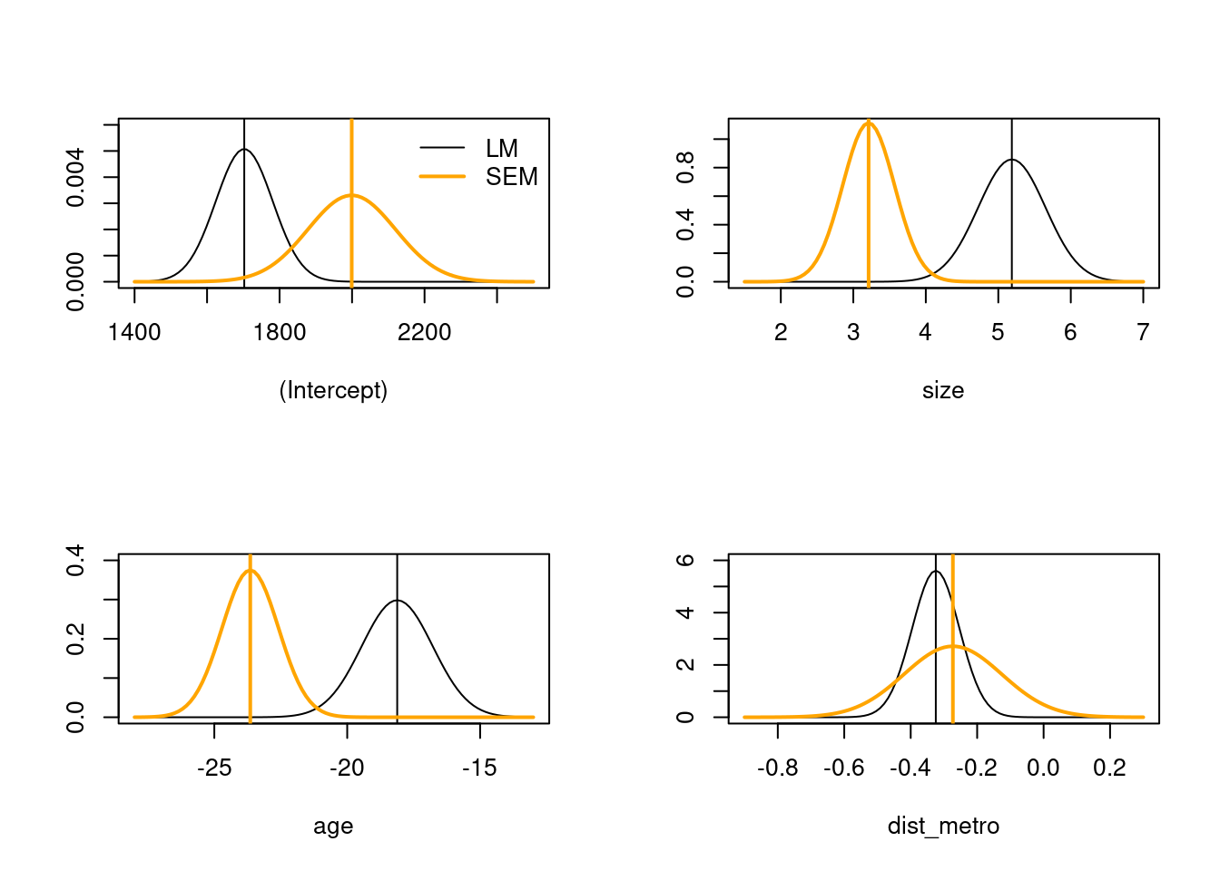
par(opar)The Hausman test also suggests mis-specification for the SEM model augmented with the municipality department level variables:
SEM_pr_md <- errorsarlm(f_pr_md, data=properties_in_dd, listw=lw, Durbin=FALSE,
    control=list(pre_eig=eigs))
summary(SEM_pr_md, Hausman=TRUE)
#
# Call:
# errorsarlm(formula = f_pr_md, data = properties_in_dd, listw = lw,
#     Durbin = FALSE, control = list(pre_eig = eigs))
#
# Residuals:
#       Min        1Q    Median        3Q       Max
# -3421.923  -320.793   -65.301   224.785  5452.101
#
# Type: error
# Coefficients: (asymptotic standard errors)
#               Estimate Std. Error  z value  Pr(>|z|)
# (Intercept) 1945.79329  333.00264   5.8432 5.121e-09
# size           3.05839    0.35711   8.5643 < 2.2e-16
# age          -23.45168    1.06301 -22.0616 < 2.2e-16
# dist_metro    -0.14969    0.13214  -1.1328    0.2573
# foreigners    -7.66310   42.72513  -0.1794    0.8577
# prgreensp     38.40538   31.36427   1.2245    0.2208
# popdens     -211.52189  190.49686  -1.1104    0.2668
# museums      -33.84713   39.33249  -0.8605    0.3895
# airbnb         0.59183    0.60062   0.9854    0.3244
#
# Lambda: 0.62414, LR test value: 335.94, p-value: < 2.22e-16
# Asymptotic standard error: 0.028289
#     z-value: 22.063, p-value: < 2.22e-16
# Wald statistic: 486.78, p-value: < 2.22e-16
#
# Log likelihood: -7836.138 for error model
# ML residual variance (sigma squared): 345330, (sigma: 587.65)
# Number of observations: 1000
# Number of parameters estimated: 11
# AIC: 15694, (AIC for lm: 16028)
# Hausman test: -1348.4, df: 9, p-value: < 2.22e-16
Extending to the SDEM models, and reporting impacts:
SDEM_pr <- errorsarlm(f_pr, data=properties_in_dd, listw=lw, Durbin=TRUE,
    control=list(pre_eig=eigs))
summary(impacts(SDEM_pr), short=TRUE, zstats=TRUE)
# Impact measures (SDEM, glht, n):
#                       Direct   Indirect       Total
# size dy/dx         3.4445402  2.0126056   5.4571458
# age dy/dx        -21.9222898 10.9931409 -10.9291489
# dist_metro dy/dx   0.2000411 -0.5494199  -0.3493789
# ========================================================
# Standard errors:
#                     Direct  Indirect     Total
# size dy/dx       0.3983375 1.0053504 1.2310345
# age dy/dx        1.1425638 2.5191830 3.1162005
# dist_metro dy/dx 0.2734082 0.3104821 0.1551602
# ========================================================
# Z-values:
#                      Direct  Indirect     Total
# size dy/dx         8.647291  2.001895  4.432976
# age dy/dx        -19.186928  4.363772 -3.507203
# dist_metro dy/dx   0.731657 -1.769570 -2.251730
#
# p-values:
#                  Direct  Indirect   Total
# size dy/dx       < 2e-16 0.045296   9.2941e-06
# age dy/dx        < 2e-16 1.2784e-05 0.00045284
# dist_metro dy/dx 0.46438 0.076799   0.02433931
we have Hausman test results still indicating strong mis-specification:
Hausman.test(SDEM_pr)
#
#   Spatial Hausman test (asymptotic)
#
# data:  NULL
# Hausman test = 53.765, df = 7, p-value = 2.618e-09
The same applies to the properties variables augmented with the municipality department level variables:
SDEM_pr_md <- errorsarlm(f_pr_md, data=properties_in_dd, listw=lw, Durbin=TRUE,
    control=list(pre_eig=eigs))
summary(impacts(SDEM_pr_md), short=TRUE, zstats=TRUE)
# Impact measures (SDEM, glht, n):
#                        Direct     Indirect       Total
# size dy/dx          3.2902831    1.6915617   4.9818448
# age dy/dx         -22.5877018    7.0789017 -15.5088001
# dist_metro dy/dx    0.2706259   -0.4643729  -0.1937470
# foreigners dy/dx  107.6194779 -146.8457503 -39.2262724
# prgreensp dy/dx    35.3436530  -12.5353740  22.8082790
# popdens dy/dx    -456.7261691  400.0782169 -56.6479522
# museums dy/dx      51.9819819  -93.3777540 -41.3957721
# airbnb dy/dx       -0.8658815    1.7162902   0.8504087
# ========================================================
# Standard errors:
#                       Direct    Indirect       Total
# size dy/dx         0.3900357   0.9742177   1.1837951
# age dy/dx          1.1250931   2.5043047   3.0554699
# dist_metro dy/dx   0.2747535   0.3097415   0.1459340
# foreigners dy/dx  87.2520047  94.9604411  45.6522625
# prgreensp dy/dx   74.3147389  79.3194509  33.1282684
# popdens dy/dx    403.5523927 439.7109652 210.7385942
# museums dy/dx     85.7152283  93.9719230  43.7578207
# airbnb dy/dx       1.1452242   1.2862740   0.6730805
# ========================================================
# Z-values:
#                       Direct   Indirect      Total
# size dy/dx         8.4358512  1.7363282  4.2083674
# age dy/dx        -20.0762965  2.8266934 -5.0757496
# dist_metro dy/dx   0.9849770 -1.4992275 -1.3276346
# foreigners dy/dx   1.2334327 -1.5463887 -0.8592405
# prgreensp dy/dx    0.4755941 -0.1580366  0.6884839
# popdens dy/dx     -1.1317642  0.9098664 -0.2688067
# museums dy/dx      0.6064498 -0.9936772 -0.9460200
# airbnb dy/dx      -0.7560803  1.3343115  1.2634575
#
# p-values:
#                  Direct  Indirect  Total
# size dy/dx       < 2e-16 0.0825058 2.5722e-05
# age dy/dx        < 2e-16 0.0047031 3.8597e-07
# dist_metro dy/dx 0.32464 0.1338146 0.18430
# foreigners dy/dx 0.21741 0.1220107 0.39021
# prgreensp dy/dx  0.63436 0.8744280 0.49115
# popdens dy/dx    0.25773 0.3628930 0.78808
# museums dy/dx    0.54422 0.3203801 0.34414
# airbnb dy/dx 0.44960 0.1821018 0.20642Hausman.test(SDEM_pr_md)
#
# Spatial Hausman test (asymptotic)
#
# data: NULL
# Hausman test = 229.24, df = 17, p-value < 2.2e-16Reaching out to the SLX models does not help, because although - as with the SDEM models - the indirect impacts (coefficients on lagged \(X\) variables) are large, so including lagged \(X\) variables especially at the properties level seems sensible, there is serious residual autocorrelation, and now the pre-test strategy points to a missing spatial process in the response:
SLX_pr <- lmSLX(f_pr, data=properties_in_dd, listw=lw, Durbin=TRUE)
summary(impacts(SLX_pr), short=TRUE, zstats=TRUE)
# Impact measures (SlX, glht, n-k):
#                       Direct   Indirect     Total
# size dy/dx         3.9424014  6.4922295 10.434631
# age dy/dx        -22.6778266 13.6377582 -9.040068
# dist_metro dy/dx   0.5710406 -0.8727816 -0.301741
# ========================================================
# Standard errors:
#                     Direct  Indirect      Total
# size dy/dx       0.4600099 0.8896271 0.90358915
# age dy/dx        1.3642232 2.1630220 2.15389898
# dist_metro dy/dx 0.3650804 0.3766962 0.07031201
# ========================================================
# Z-values:
#                      Direct  Indirect     Total
# size dy/dx         8.570254  7.297698 11.547982
# age dy/dx        -16.623252  6.304956 -4.197072
# dist_metro dy/dx   1.564150 -2.316938 -4.291458
#
# p-values:
#                  Direct  Indirect   Total
# size dy/dx       < 2e-16 2.9265e-13 < 2.22e-16
# age dy/dx        < 2e-16 2.8828e-10 2.7039e-05
# dist_metro dy/dx 0.11778 0.020507 1.7750e-05spdep::lm.morantest(SLX_pr, lw)
#
# Global Moran I for regression residuals
#
# data:
# model: lm(formula = formula(paste("y ~ ",
# paste(colnames(x)[-1], collapse = "+"))), data =
# as.data.frame(x), weights = weights)
# weights: lw
#
# Moran I statistic standard deviate = 24.275, p-value <
# 2.2e-16
# alternative hypothesis: greater
# sample estimates:
# Observed Moran I Expectation Variance
# 0.4505572652 -0.0029076149 0.0003489564if (packageVersion("spdep") < "1.3.3") {
spdep::lm.LMtests(SLX_pr, lw, test=c("RLMerr", "RLMlag"))
} else {
spdep::lm.RStests(SLX_pr, lw, test=c("adjRSerr", "adjRSlag"))
}
#
# Rao's score (a.k.a Lagrange multiplier) diagnostics for
# spatial dependence
#
# data:
# model: lm(prpsqm ~ size + age + dist_metro + lag.size +
# lag.age + lag.dist_metro, data = properties_in_dd, listw =
# lw)
# test weights: lw
#
# adjRSerr = 3.9929, df = 1, p-value = 0.04569
#
#
# Rao's score (a.k.a Lagrange multiplier) diagnostics for
# spatial dependence
#
# data:
# model: lm(prpsqm ~ size + age + dist_metro + lag.size +
# lag.age + lag.dist_metro, data = properties_in_dd, listw =
# lw)
# test weights: lw
#
# adjRSlag = 54.185, df = 1, p-value = 1.825e-13SLX_pr_md <- lmSLX(f_pr_md, data=properties_in_dd, listw=lw, Durbin=TRUE)
summary(impacts(SLX_pr_md), short=TRUE, zstats=TRUE)
# Impact measures (SlX, glht, n-k):
# Direct Indirect Total
# size dy/dx 3.6899279 5.1853598 8.8752878
# age dy/dx -22.4862582 7.7433691 -14.7428891
# dist_metro dy/dx 0.4883417 -0.6216376 -0.1332958
# foreigners dy/dx 111.8693211 -144.2912677 -32.4219466
# prgreensp dy/dx -7.9374540 33.7296361 25.7921821
# popdens dy/dx -175.9679694 76.3367323 -99.6312371
# museums dy/dx 132.9274926 -150.5428303 -17.6153377
# airbnb dy/dx -1.6203107 2.0992718 0.4789610
# ========================================================
# Standard errors:
# Direct Indirect Total
# size dy/dx 0.4374870 0.8640075 0.88540694
# age dy/dx 1.2999436 2.1706052 2.20258646
# dist_metro dy/dx 0.3469593 0.3606514 0.07353124
# foreigners dy/dx 113.3256387 115.6423334 22.69480121
# prgreensp dy/dx 98.1127344 99.5966256 16.36663957
# popdens dy/dx 521.4661878 532.2960996 105.63203070
# museums dy/dx 115.4990904 118.1243717 21.60621836
# airbnb dy/dx 1.5181784 1.5638933 0.33577968
# ========================================================
# Z-values:
# Direct Indirect Total
# size dy/dx 8.43437158 6.0015219 10.0239645
# age dy/dx -17.29787276 3.5673779 -6.6934440
# dist_metro dy/dx 1.40748996 -1.7236520 -1.8127784
# foreigners dy/dx 0.98714927 -1.2477374 -1.4286068
# prgreensp dy/dx -0.08090136 0.3386624 1.5758997
# popdens dy/dx -0.33744847 0.1434103 -0.9431915
# museums dy/dx 1.15089645 -1.2744434 -0.8152902
# airbnb dy/dx -1.06727292 1.3423369 1.4264145
#
# p-values:
# Direct Indirect Total
# size dy/dx < 2e-16 1.9548e-09 < 2.22e-16
# age dy/dx < 2e-16 0.00036057 2.1798e-11
# dist_metro dy/dx 0.15928 0.08477068 0.069866
# foreigners dy/dx 0.32357 0.21212723 0.153117
# prgreensp dy/dx 0.93552 0.73486404 0.115049
# popdens dy/dx 0.73578 0.88596617 0.345583
# museums dy/dx 0.24977 0.20250631 0.414906
# airbnb dy/dx 0.28585 0.17948677 0.153749spdep::lm.morantest(SLX_pr_md, lw)
#
# Global Moran I for regression residuals
#
# data:
# model: lm(formula = formula(paste("y ~ ",
# paste(colnames(x)[-1], collapse = "+"))), data =
# as.data.frame(x), weights = weights)
# weights: lw
#
# Moran I statistic standard deviate = 22.047, p-value <
# 2.2e-16
# alternative hypothesis: greater
# sample estimates:
# Observed Moran I Expectation Variance
# 0.3978202243 -0.0070160067 0.0003371825if (packageVersion("spdep") < "1.3.3") {
spdep::lm.LMtests(SLX_pr_md, lw, test=c("RLMerr", "RLMlag"))
} else {
spdep::lm.RStests(SLX_pr_md, lw, test=c("adjRSerr", "adjRSlag"))
}
#
# Rao's score (a.k.a Lagrange multiplier) diagnostics for
# spatial dependence
#
# data:
# model: lm(prpsqm ~ size + age + dist_metro + foreigners +
# prgreensp + popdens + museums + airbnb + lag.size + lag.age
# + lag.dist_metro + lag.foreigners + lag.prgreensp +
# lag.popdens + lag.museums + lag.airbnb, data =
# properties_in_dd, listw = lw)
# test weights: lw
#
# adjRSerr = 15.011, df = 1, p-value = 0.0001069
#
#
# Rao's score (a.k.a Lagrange multiplier) diagnostics for
# spatial dependence
#
# data:
# model: lm(prpsqm ~ size + age + dist_metro + foreigners +
# prgreensp + popdens + museums + airbnb + lag.size + lag.age
# + lag.dist_metro + lag.foreigners + lag.prgreensp +
# lag.popdens + lag.museums + lag.airbnb, data =
# properties_in_dd, listw = lw)
# test weights: lw
#
# adjRSlag = 56.758, df = 1, p-value = 4.929e-14So on balance, the pre-test strategy has not worked out too well; it is unclear what is missing in the model.
Exercise 17.4
Turning to estimating the general nested model first, followed by excluding the Durbin (spatially lagged \(X\)) variables, a likelihood ratio test shows that the spatially lagged \(X\) variables should be retained in the model:
lmtest::lrtest(SARAR_pr, GNM_pr)
# Likelihood ratio test
#
# Model 1: prpsqm ~ size + age + dist_metro
# Model 2: prpsqm ~ size + age + dist_metro
#   #Df  LogLik Df  Chisq Pr(>Chisq)
# 1   7 -7814.6
# 2  10 -7783.9  3 61.303  3.096e-13 ***
# ---
# Signif. codes:  0 '***' 0.001 '**' 0.01 '*' 0.05 '.' 0.1 ' ' 1
Again using a likelihood ratio test, the GNM model outperforms the SDEM model:
lmtest::lrtest(SDEM_pr, GNM_pr)
# Likelihood ratio test
#
# Model 1: prpsqm ~ size + age + dist_metro
# Model 2: prpsqm ~ size + age + dist_metro
#   #Df  LogLik Df Chisq Pr(>Chisq)
# 1   9 -7850.3
# 2  10 -7783.9  1 132.7  < 2.2e-16 ***
# ---
# Signif. codes: 0 '***' 0.001 '**' 0.01 '*' 0.05 '.' 0.1 ' ' 1as is also the case with the SDM model:
lmtest::lrtest(SDM_pr, GNM_pr)
# Likelihood ratio test
#
# Model 1: prpsqm ~ size + age + dist_metro
# Model 2: prpsqm ~ size + age + dist_metro
#   #Df  LogLik Df  Chisq Pr(>Chisq)
# 1   9 -7842.4
# 2  10 -7783.9  1 117.06  < 2.2e-16 ***
# ---
# Signif. codes:  0 '***' 0.001 '**' 0.01 '*' 0.05 '.' 0.1 ' ' 1
and the SLX model:
lmtest::lrtest(SLX_pr, GNM_pr)
# Warning in modelUpdate(objects[[i - 1]], objects[[i]]): original
# model was of class "SlX", updated model is of class "Sarlm"
# Likelihood ratio test
#
# Model 1: y ~ size + age + dist_metro + lag.size + lag.age + lag.dist_metro
# Model 2: prpsqm ~ size + age + dist_metro
#   #Df  LogLik Df  Chisq Pr(>Chisq)
# 1   8 -8040.1
# 2  10 -7783.9  2 512.46  < 2.2e-16 ***
# ---
# Signif. codes:  0 '***' 0.001 '**' 0.01 '*' 0.05 '.' 0.1 ' ' 1
Is the inclusion of the municipality department level variables in the GNM model justified?
No, not really:
lmtest::lrtest(GNM_pr, GNM_pr_md)
# Likelihood ratio test
#
# Model 1: prpsqm ~ size + age + dist_metro
# Model 2: prpsqm ~ size + age + dist_metro + foreigners + prgreensp + popdens +
#     museums + airbnb
#   #Df  LogLik Df  Chisq Pr(>Chisq)
# 1  10 -7783.9
# 2  20 -7773.4 10 20.956     0.0214 *
# ---
# Signif. codes:  0 '***' 0.001 '**' 0.01 '*' 0.05 '.' 0.1 ' ' 1
If we drop the municipality department level variables from the Durbin term, we lose fewer degrees of freedom, so preferring the model including the municipality department level variables:
lmtest::lrtest(GNM_pr, GNM_pr_md1)
# Likelihood ratio test
#
# Model 1: prpsqm ~ size + age + dist_metro
# Model 2: prpsqm ~ size + age + dist_metro + foreigners + prgreensp + popdens +
#     museums + airbnb
#   #Df  LogLik Df  Chisq Pr(>Chisq)
# 1  10 -7783.9
# 2  15 -7775.5  5 16.794   0.004908 **
# ---
# Signif. codes:  0 '***' 0.001 '**' 0.01 '*' 0.05 '.' 0.1 ' ' 1
Unfortunately, impacts are depressing here:
trs <- trW(as(lw, "CsparseMatrix"))
i_GNM_pr_md1 <- impacts(GNM_pr_md1, tr=trs, R=2000)
summary(i_GNM_pr_md1, short=TRUE, zstats=TRUE)
# Impact measures (sacmixed, trace):
#                        Direct    Indirect        Total
# size dy/dx         3.23740995   7.2985861   10.5359961
# age dy/dx        -23.03565197  10.9935858  -12.0420662
# dist_metro dy/dx   0.26484655  -0.4603147   -0.1954681
# foreigners dy/dx  -5.71030959 -23.1783890  -28.8886986
# prgreensp dy/dx    5.63045876  22.8542711   28.4847299
# popdens dy/dx    -20.87711879 -84.7411115 -105.6182302
# museums dy/dx     -4.03610471 -16.3827204  -20.4188251
# airbnb dy/dx       0.09458806   0.3839369    0.4785250
# ========================================================
# Simulation results ( variance matrix):
# ========================================================
# Simulated standard errors
#                      Direct    Indirect       Total
# size dy/dx        0.3640421   2.6190738   2.7467624
# age dy/dx         1.0609491   6.2160972   6.5935134
# dist_metro dy/dx  0.2184669   0.3088026   0.1951595
# foreigners dy/dx 12.0221664  49.7510511  61.7196283
# prgreensp dy/dx   8.6198780  35.3964918  43.9720658
# popdens dy/dx    55.5472638 229.0887514 284.4003045
# museums dy/dx    11.0348774  45.6325914  56.6243048
# airbnb dy/dx      0.1748009   0.7225902   0.8965895
#
# Simulated z-values:
#                       Direct   Indirect      Total
# size dy/dx         8.9133828  2.8209650  3.8711621
# age dy/dx        -21.6863110  1.7493508 -1.8402838
# dist_metro dy/dx   1.1398599 -1.4287514 -0.9847357
# foreigners dy/dx  -0.4394990 -0.4333881 -0.4349547
# prgreensp dy/dx    0.6686783  0.6573043  0.6601962
# popdens dy/dx     -0.4087387 -0.3995878 -0.4017063
# museums dy/dx     -0.3438904 -0.3398924 -0.3409306
# airbnb dy/dx       0.5116462  0.5053584  0.5070361
#
# Simulated p-values:
#                  Direct  Indirect  Total
# size dy/dx       < 2e-16 0.0047879 0.00010832
# age dy/dx        < 2e-16 0.0802304 0.06572658
# dist_metro dy/dx 0.25434 0.1530757 0.32475393
# foreigners dy/dx 0.66030 0.6647328 0.66359528
# prgreensp dy/dx  0.50370 0.5109853 0.50912793
# popdens dy/dx    0.68273 0.6894601 0.68790019
# museums dy/dx    0.73093 0.7339376 0.73315583
# airbnb dy/dx     0.60890 0.6133071 0.61212948
The values and standard errors of the spatial coefficients suggest numerical problems in finding an optimum where the two coefficients are equally strong but with opposing signs:
c("response"=GNM_pr_md1$rho, "response se"=GNM_pr_md1$rho.se, "residual"=GNM_pr_md1$lambda, "residual se"=GNM_pr_md1$lambda.se)
#    response.rho     response se residual.lambda     residual se
#      0.85971901      0.01547632     -0.86679315      0.04377824
If we fall back on the properties level only GNM, total impacts are only significant in conventional terms for size:
i_GNM_pr <- impacts(GNM_pr, tr=trs, R=2000)
summary(i_GNM_pr, short=TRUE, zstats=TRUE)
# Impact measures (sacmixed, trace):
#                       Direct   Indirect     Total
# size dy/dx         3.3625439  9.2475200 12.610064
# age dy/dx        -22.7517496 16.8353069 -5.916443
# dist_metro dy/dx   0.2927224 -0.6523253 -0.359603
# ========================================================
# Simulation results ( variance matrix):
# ========================================================
# Simulated standard errors
#                     Direct  Indirect     Total
# size dy/dx       0.3727683 2.8632782 3.0123731
# age dy/dx        1.0699884 6.5316350 6.8967868
# dist_metro dy/dx 0.2179827 0.3066225 0.2007306
#
# Simulated z-values:
#                      Direct  Indirect      Total
# size dy/dx         9.025316  3.201576  4.1599609
# age dy/dx        -21.250479  2.577098 -0.8562105
# dist_metro dy/dx   1.331723 -2.102057 -1.7647792
#
# Simulated p-values:
#                  Direct  Indirect  Total
# size dy/dx       < 2e-16 0.0013668 3.183e-05
# age dy/dx        < 2e-16 0.0099634 0.391881
# dist_metro dy/dx 0.18295 0.0355483 0.077601
The same problem occurs without the municipality department level variables; the impacts are being driven by the large spatial coefficient on the lagged response:
c("response"=GNM_pr$rho, "response se"=GNM_pr$rho.se, "residual"=GNM_pr$lambda, "residual se"=GNM_pr$lambda.se)
#    response.rho     response se residual.lambda     residual se
#      0.88013827      0.01319649     -0.89698377      0.03914228
Exercise 17.5
We cannot say that the spatial econometrics approach has reached a clear conclusion. When including the upper level variables, we introduce a lot of spatial autocorrelation at the lower level. It is arguable that the MRF random effect at the upper level and including only the properties level variables gets at least as far as the most complex spatial econometrics models. It is fairly clear that mapping the actual green space and museums, and measuring distance from each property to the attractions would remove the scale problem for those variables. Disaggregation of the foreigners, airbnb and population density variables would be highly desirable. With improvements to the properties level data set, including more variables describing the properties themselves, much of the mis-specification should be removed.
sessionInfo()
# R version 4.6.0 (2026-04-24)
# Platform: x86_64-pc-linux-gnu
# Running under: Ubuntu 24.04.4 LTS
#
# Matrix products: default
# BLAS:   /usr/lib/x86_64-linux-gnu/openblas-pthread/libblas.so.3
# LAPACK: /usr/lib/x86_64-linux-gnu/openblas-pthread/libopenblasp-r0.3.26.so;  LAPACK version 3.12.0
#
# locale:
#  [1] LC_CTYPE=en_US.UTF-8       LC_NUMERIC=C
#  [3] LC_TIME=en_GB.UTF-8        LC_COLLATE=en_US.UTF-8
#  [5] LC_MONETARY=en_GB.UTF-8    LC_MESSAGES=en_US.UTF-8
#  [7] LC_PAPER=en_GB.UTF-8       LC_NAME=C
#  [9] LC_ADDRESS=C               LC_TELEPHONE=C
# [11] LC_MEASUREMENT=en_GB.UTF-8 LC_IDENTIFICATION=C
#
# time zone: Europe/Berlin
# tzcode source: system (glibc)
#
# attached base packages:
# [1] stats     graphics  grDevices utils     datasets  methods
# [7] base
#
# other attached packages:
# [1] spatialreg_1.4-3 Matrix_1.7-5     spdep_1.4-2
# [4] sf_1.1-1         spData_2.3.5
#
# loaded via a namespace (and not attached):
#  [1] jsonlite_2.0.0         compiler_4.6.0
#  [3] Rcpp_1.1.1-1.1         marginaleffects_0.32.0
#  [5] splines_4.6.0          boot_1.3-32
#  [7] fastmap_1.2.0          TH.data_1.1-5
#  [9] lattice_0.22-9         coda_0.19-4.1
# [11] deldir_2.0-4           generics_0.1.4
# [13] lmtest_0.9-40          classInt_0.4-11
# [15] s2_1.1.9               knitr_1.51
# [17] backports_1.5.1        MASS_7.3-65
# [19] htmlwidgets_1.6.4      units_1.0-1
# [21] LearnBayes_2.15.2      DBI_1.3.0
# [23] rlang_1.2.0            multcomp_1.4-30
# [25] sp_2.2-1               xfun_0.57
# [27] otel_0.2.0             spDataLarge_2.1.2
# [29] cli_3.6.6              mgcv_1.9-4
# [31] class_7.3-23           wk_0.9.5
# [33] digest_0.6.39          grid_4.6.0
# [35] mvtnorm_1.3-7          sandwich_3.1-1
# [37] nlme_3.1-169           KernSmooth_2.23-26
# [39] data.table_1.18.2.1    proxy_0.4-29
# [41] evaluate_1.0.5         codetools_0.2-20
# [43] zoo_1.8-15             stats4_4.6.0
# [45] survival_3.8-6         e1071_1.7-17
# [47] rmarkdown_2.31         tools_4.6.0
# [49] htmltools_0.5.9