8  Plotting

Exercise 8.1

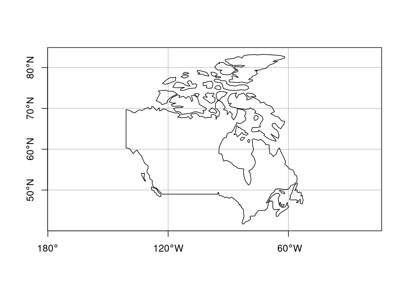
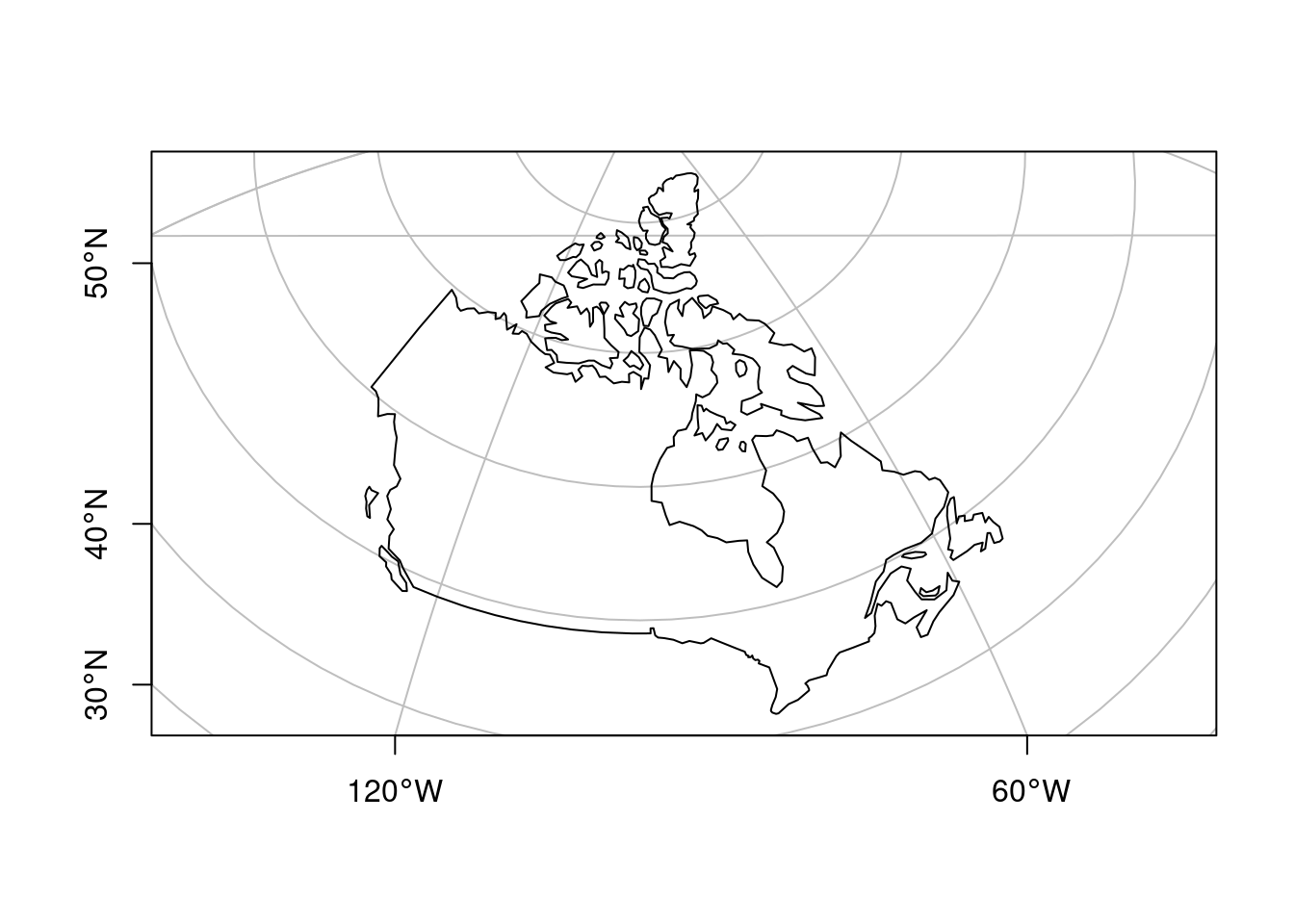
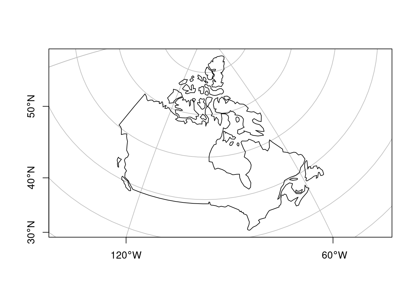
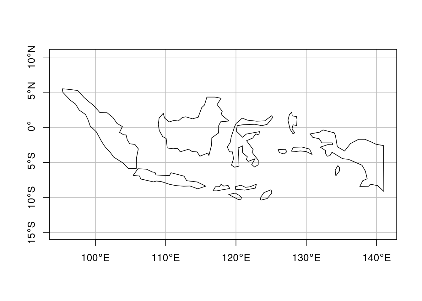
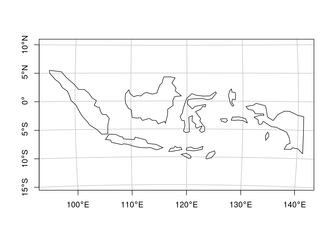
For the countries Indonesia and Canada, create individual plots using equirectangular, orthographic, and Lambert equal area projections, while choosing projection parameters sensible for the area.

# +proj=eqc +lat_ts=0 +lat_0=0 +lon_0=0 +x_0=0 +y_0=0 +ellps=WGS84 +units=m
# +proj=ortho +lon_0=0 +lat_0=0
# +proj=laea +lon_0=0 +lat_0=0
library(sf)
# Linking to GEOS 3.12.2, GDAL 3.11.4, PROJ 9.4.1; sf_use_s2() is
# TRUE
library(tidyverse)
# ── Attaching core tidyverse packages ──────────── tidyverse 2.0.0 ──
# ✔ dplyr     1.2.1     ✔ readr     2.2.0
# ✔ forcats   1.0.1     ✔ stringr   1.6.0
# ✔ ggplot2   4.0.3     ✔ tibble    3.3.1
# ✔ lubridate 1.9.5     ✔ tidyr     1.3.2
# ✔ purrr     1.2.2
# ── Conflicts ────────────────────────────── tidyverse_conflicts() ──
# ✖ dplyr::filter() masks stats::filter()
# ✖ dplyr::lag()    masks stats::lag()
# ℹ Use the conflicted package (<http://conflicted.r-lib.org/>) to force all conflicts to become errors
library(rnaturalearth)
ne = ne_countries(returnclass = "sf")
ne |> filter(admin == "Canada") -> ca
ne |> filter(admin == "Indonesia") -> ind
st_geometry(ca) |> st_centroid()
# Geometry set for 1 feature 
# Geometry type: POINT
# Dimension:     XY
# Bounding box:  xmin: -96.39551 ymin: 60.47676 xmax: -96.39551 ymax: 60.47676
# Geodetic CRS:  WGS 84
# POINT (-96.39551 60.47676)
ca_eqc = st_crs("+proj=eqc +lat_ts=60.6")
st_geometry(ca) |> st_transform(ca_eqc) |> plot(axes=TRUE, graticule =TRUE)

ca_ortho = st_crs("+proj=ortho +lat_0=60.6 +lon_0=-96.4")
st_geometry(ca) |> st_transform(ca_ortho) |> plot(axes=TRUE, graticule=TRUE)

ca_laea = st_crs("+proj=laea +lat_0=60.6 +lon_0=-96.4")
st_geometry(ca) |> st_transform(ca_laea) |> plot(axes=TRUE, graticule=TRUE)

st_geometry(ind) |> st_centroid()
# Geometry set for 1 feature 
# Geometry type: POINT
# Dimension:     XY
# Bounding box:  xmin: 117.3629 ymin: -2.271715 xmax: 117.3629 ymax: -2.271715
# Geodetic CRS:  WGS 84
# POINT (117.3629 -2.271715)
in_eqc = st_crs("+proj=eqc +lat_ts=-2.3")
st_geometry(ind) |> st_transform(in_eqc) |> plot(axes=TRUE, graticule =TRUE)

in_ortho = st_crs("+proj=ortho +lat_0=-2.3 +lon_0=117")
st_geometry(ind) |> st_transform(in_ortho) |> plot(axes=TRUE, graticule=TRUE)

in_laea = st_crs("+proj=laea +lat_0=-2.3 +lon_0=117")
st_geometry(ind) |> st_transform(in_laea) |> plot(axes=TRUE, graticule=TRUE)

Exercise 8.2

Recreate the plot in Figure 8.3 with ggplot2 and with tmap.

ggplot2:

library(sf)
nc <- read_sf(system.file("gpkg/nc.gpkg", package = "sf"))
b = st_buffer(nc[1,1], units::set_units(10, km)) |> st_cast("LINESTRING")
# Warning in st_cast.sf(st_buffer(nc[1, 1], units::set_units(10,
# km)), "LINESTRING"): repeating attributes for all sub-geometries
# for which they may not be constant
library(ggplot2)
ggplot() + geom_sf(data = nc, aes(fill = BIR74)) +
        geom_sf(data = b, mapping = aes(colour = 'red')) +
        scale_fill_gradientn(colours = sf.colors())

tmap: see https://r-tmap.github.io/tmap-book/

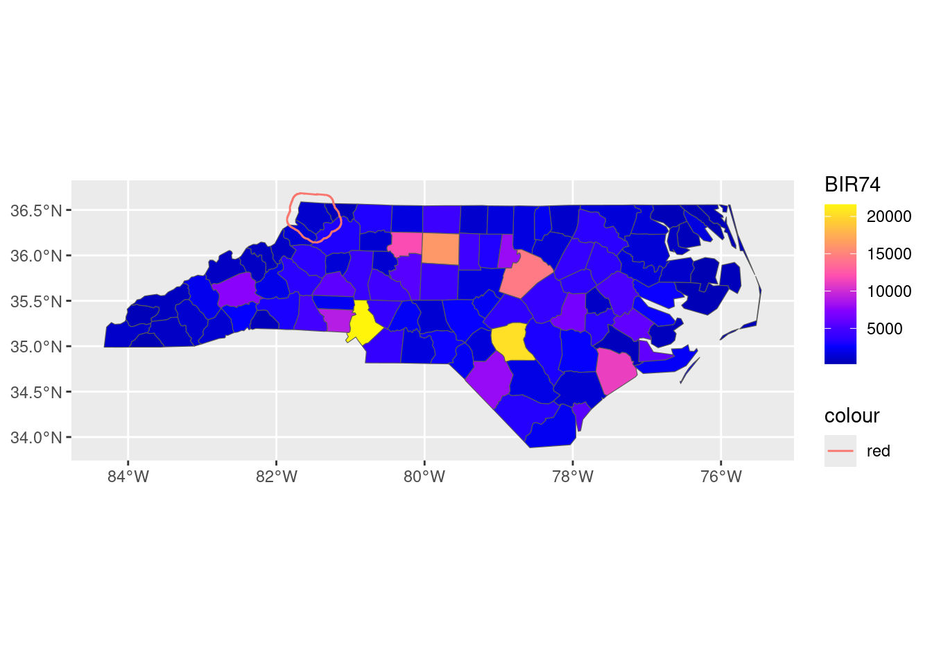
library(tmap)
b = st_buffer(nc[1,1], units::set_units(10, km)) |> st_cast("LINESTRING")
# Warning in st_cast.sf(st_buffer(nc[1, 1], units::set_units(10,
# km)), "LINESTRING"): repeating attributes for all sub-geometries
# for which they may not be constant
tm_shape(nc) + 
    tm_polygons("BIR74", title = "BIR74") + 
    tm_layout(legend.outside=TRUE) +
    tm_shape(b) +
    tm_lines(legend.lwd.show = FALSE, col = 'red')
# 
# ── tmap v3 code detected ───────────────────────────────────────────
# [v3->v4] `tm_polygons()`: migrate the argument(s) related to the
# legend of the visual variable `fill` namely 'title' to 'fill.legend
# = tm_legend(<HERE>)'
# [v3->v4] `tm_lines()`: use `lwd.legend = tm_legend_hide()` instead
# of `legend.lwd.show = FALSE`.

Exercise 8.3

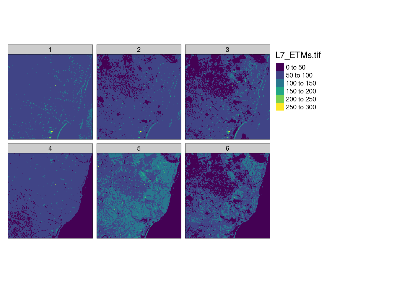
Recreate the plot in Figure 8.7 using the viridis colour ramp.

library(stars)
# Loading required package: abind
library(viridis)
# Loading required package: viridisLite
r <- read_stars(system.file("tif/L7_ETMs.tif", package = "stars"))
tm_shape(r) + tm_raster(palette = viridis(100))
# 
# ── tmap v3 code detected ───────────────────────────────────────────
# [v3->v4] `tm_tm_raster()`: migrate the argument(s) related to the
# scale of the visual variable `col` namely 'palette' (rename to
# 'values') to col.scale = tm_scale(<HERE>).

Exercise 8.4

View the interactive plot in Figure 8.7 using the “view” (interactive) mode of tmap, and explore which interactions are possible;

library(stars)
library(viridis)
r <- read_stars(system.file("tif/L7_ETMs.tif", package = "stars"))
tmap_mode("view")
# ℹ tmap modes "plot" - "view"
# ℹ toggle with `tmap::ttm()`
tm_shape(r) + tm_raster(palette = viridis(100))
# 
# ── tmap v3 code detected ───────────────────────────────────────────
# [v3->v4] `tm_tm_raster()`: migrate the argument(s) related to the
# scale of the visual variable `col` namely 'palette' (rename to
# 'values') to col.scale = tm_scale(<HERE>).

Interactions: zoom, pan, linked cursor.

Also explore adding + tm_facets(as.layers=TRUE) and try switching layers on and off.

tmap_mode("view")
# ℹ tmap modes "plot" - "view"
tm_shape(r) + tm_raster(palette = viridis(100)) + 
        tm_facets(as.layers=TRUE)
# 
# ── tmap v3 code detected ───────────────────────────────────────────
# [v3->v4] `tm_tm_raster()`: migrate the argument(s) related to the
# scale of the visual variable `col` namely 'palette' (rename to
# 'values') to col.scale = tm_scale(<HERE>).

Layer switch on left-hand side (layer symbol).

Try also setting a transparency value to 0.5.

tmap_mode("view")
# ℹ tmap modes "plot" - "view"
tm_shape(r) + tm_raster(palette = viridis(100), alpha = .5) + 
        tm_facets(as.layers=TRUE)
# 
# ── tmap v3 code detected ───────────────────────────────────────────
# [v3->v4] `tm_tm_raster()`: migrate the argument(s) related to the
# scale of the visual variable `col` namely 'palette' (rename to
# 'values') to col.scale = tm_scale(<HERE>).[v3->v4] `tm_raster()`: use `col_alpha` instead of `alpha`.

This shows the base map shining through transparent raster colors (switch 3 of the 4 layers off to see this).